

6.10 Transfer Matrix Method
207
or
{Z }
R
i = [U ] i {Z }
L
i
(6.68)
[U ] i is referred to as point transfer matrix, as it relates the two adjacent state vectors
over a point.
6.10.1 Transfer Matrices as a Means of Elimination
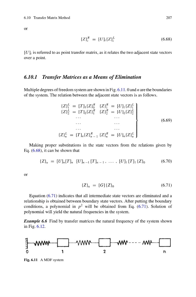
Multiple degrees of freedom system are shown in Fig. 6.11. 0 and n are the boundaries
of the system. The relation between the adjacent state vectors is as follows.
{Z }
L
1 = [T ] 1 {Z }
R
0
{Z }
R
1 = [U ] 1 {Z }
L
1
{Z }
L
2 = [T ] 2 {Z }
R
1
{Z }
R
2 = [U ] 2 {Z }
L
2
· · ·
· · ·
· · ·
· · ·
· · ·
· · ·
{Z }
L
n = [T ] n {Z }
R
n − 1 {Z }
R
n = [U ] n {Z }
L
n
⎫
⎪ ⎪ ⎪ ⎪ ⎪ ⎪ ⎪ ⎬
⎪ ⎪ ⎪ ⎪ ⎪ ⎪ ⎪ ⎭
(6.69)
Making proper substitutions in the state vectors from the relations given by
Eq. (6.68), it can be shown that
{Z } n = [U ] n [T ] n [U ] n −1 [T ] n − 1 , . . . , [U ] 1 [T ] 1 {Z } 0
(6.70)
or
{Z } n = [G] {Z } 0
(6.71)
Equation (6.71) indicates that all intermediate state vectors are eliminated and a
relationship is obtained between boundary state vectors. After putting the boundary
conditions, a polynomial in p
2 will be obtained from Eq. (6.71). Solution of
polynomial will yield the natural frequencies in the system.
Example 6.6 Find by transfer matrices the natural frequency of the system shown
in Fig. 6.12.
Fig. 6.11 A MDF system
207
or
{Z }
R
i = [U ] i {Z }
L
i
(6.68)
[U ] i is referred to as point transfer matrix, as it relates the two adjacent state vectors
over a point.
6.10.1 Transfer Matrices as a Means of Elimination
Multiple degrees of freedom system are shown in Fig. 6.11. 0 and n are the boundaries
of the system. The relation between the adjacent state vectors is as follows.
{Z }
L
1 = [T ] 1 {Z }
R
0
{Z }
R
1 = [U ] 1 {Z }
L
1
{Z }
L
2 = [T ] 2 {Z }
R
1
{Z }
R
2 = [U ] 2 {Z }
L
2
· · ·
· · ·
· · ·
· · ·
· · ·
· · ·
{Z }
L
n = [T ] n {Z }
R
n − 1 {Z }
R
n = [U ] n {Z }
L
n
⎫
⎪ ⎪ ⎪ ⎪ ⎪ ⎪ ⎪ ⎬
⎪ ⎪ ⎪ ⎪ ⎪ ⎪ ⎪ ⎭
(6.69)
Making proper substitutions in the state vectors from the relations given by
Eq. (6.68), it can be shown that
{Z } n = [U ] n [T ] n [U ] n −1 [T ] n − 1 , . . . , [U ] 1 [T ] 1 {Z } 0
(6.70)
or
{Z } n = [G] {Z } 0
(6.71)
Equation (6.71) indicates that all intermediate state vectors are eliminated and a
relationship is obtained between boundary state vectors. After putting the boundary
conditions, a polynomial in p
2 will be obtained from Eq. (6.71). Solution of
polynomial will yield the natural frequencies in the system.
Example 6.6 Find by transfer matrices the natural frequency of the system shown
in Fig. 6.12.
Fig. 6.11 A MDF system