

152
4 Numerical Methods in Structural Dynamics …
Therefore, the computational recipe can be expressed as
F(ω n ) =
1
2
Y n + W
n
N Z n
F
ω n + N /2
=
1
2
Y n − W
n
N Z n
(4.61)
for n = 0, 1, 2, . . . ,
N
2
− 1
.
The above form exists in most of the FFT programmes.
Exercises
4.1. A SDF system has k = 7150 N/m and the mass is 20 kg. Determine the
response of the mass by numerical integration, if an external force F (t) =
50 cos (10t) is applied to the system. The system is undamped and is initially
at rest.
4.2. Solve Prob. 4.1 by applying Newmark’s β-method using β =1/5.
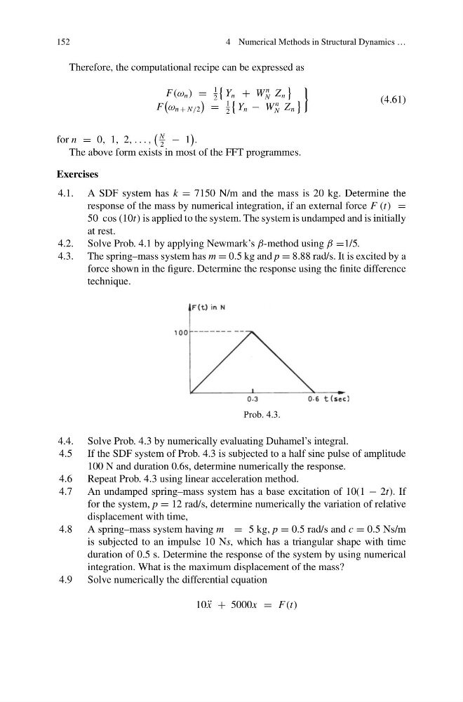
4.3. The spring–mass system has m = 0.5 kg and p = 8.88 rad/s. It is excited by a
force shown in the figure. Determine the response using the finite difference
technique.
Prob. 4.3.
4.4. Solve Prob. 4.3 by numerically evaluating Duhamel’s integral.
4.5 If the SDF system of Prob. 4.3 is subjected to a half sine pulse of amplitude
100 N and duration 0.6s, determine numerically the response.
4.6 Repeat Prob. 4.3 using linear acceleration method.
4.7 An undamped spring–mass system has a base excitation of 10(1 − 2t). If
for the system, p = 12 rad/s, determine numerically the variation of relative
displacement with time,
4.8 A spring–mass system having m = 5 kg, p = 0.5 rad/s and c = 0.5 Ns/m
is subjected to an impulse 10 Ns, which has a triangular shape with time
duration of 0.5 s. Determine the response of the system by using numerical
integration. What is the maximum displacement of the mass?
4.9 Solve numerically the differential equation
10 ¨
x + 5000x = F(t)
4 Numerical Methods in Structural Dynamics …
Therefore, the computational recipe can be expressed as
F(ω n ) =
1
2
Y n + W
n
N Z n
F
ω n + N /2
=
1
2
Y n − W
n
N Z n
(4.61)
for n = 0, 1, 2, . . . ,
N
2
− 1
.
The above form exists in most of the FFT programmes.
Exercises
4.1. A SDF system has k = 7150 N/m and the mass is 20 kg. Determine the
response of the mass by numerical integration, if an external force F (t) =
50 cos (10t) is applied to the system. The system is undamped and is initially
at rest.
4.2. Solve Prob. 4.1 by applying Newmark’s β-method using β =1/5.
4.3. The spring–mass system has m = 0.5 kg and p = 8.88 rad/s. It is excited by a
force shown in the figure. Determine the response using the finite difference
technique.
Prob. 4.3.
4.4. Solve Prob. 4.3 by numerically evaluating Duhamel’s integral.
4.5 If the SDF system of Prob. 4.3 is subjected to a half sine pulse of amplitude
100 N and duration 0.6s, determine numerically the response.
4.6 Repeat Prob. 4.3 using linear acceleration method.
4.7 An undamped spring–mass system has a base excitation of 10(1 − 2t). If
for the system, p = 12 rad/s, determine numerically the variation of relative
displacement with time,
4.8 A spring–mass system having m = 5 kg, p = 0.5 rad/s and c = 0.5 Ns/m
is subjected to an impulse 10 Ns, which has a triangular shape with time
duration of 0.5 s. Determine the response of the system by using numerical
integration. What is the maximum displacement of the mass?
4.9 Solve numerically the differential equation
10 ¨
x + 5000x = F(t)