

148
4 Numerical Methods in Structural Dynamics …
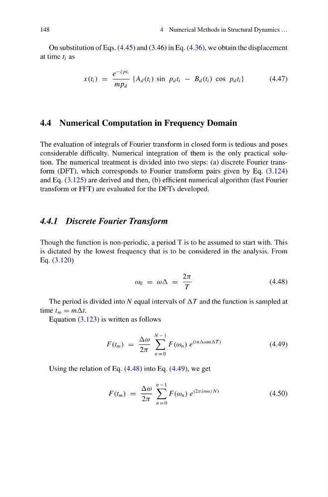
On substitution of Eqs. (4.45) and (3.46) in Eq. (4.36), we obtain the displacement
at time t i as
x(t i ) =
e
−ζ pt i
mp d
{A d (t i ) sin p d t i − B d (t i ) cos p d t i }
(4.47)
4.4 Numerical Computation in Frequency Domain
The evaluation of integrals of Fourier transform in closed form is tedious and poses
considerable difficulty. Numerical integration of them is the only practical solution. The numerical treatment is divided into two steps: (a) discrete Fourier transform (DFT), which corresponds to Fourier transform pairs given by Eq. (3.124)
and Eq. (3.125) are derived and then, (b) efficient numerical algorithm (fast Fourier
transform or FFT) are evaluated for the DFTs developed.
4.4.1 Discrete Fourier Transform
Though the function is non-periodic, a period T is to be assumed to start with. This
is dictated by the lowest frequency that is to be considered in the analysis. From
Eq. (3.120)
ω 0 = ωω =
2π
T
(4.48)
The period is divided into N equal intervals of T and the function is sampled at
time t m = mt.
Equation (3.123) is written as follows
F(t m ) =
ω
2π
N − 1
n = 0
F(ω n ) e
(inωmT )
(4.49)
Using the relation of Eq. (4.48) into Eq. (4.49), we get
F(t m ) =
ω
2π
n − 1
n = 0
F(ω n ) e
(2πinm/N )
(4.50)
4 Numerical Methods in Structural Dynamics …
On substitution of Eqs. (4.45) and (3.46) in Eq. (4.36), we obtain the displacement
at time t i as
x(t i ) =
e
−ζ pt i
mp d
{A d (t i ) sin p d t i − B d (t i ) cos p d t i }
(4.47)
4.4 Numerical Computation in Frequency Domain
The evaluation of integrals of Fourier transform in closed form is tedious and poses
considerable difficulty. Numerical integration of them is the only practical solution. The numerical treatment is divided into two steps: (a) discrete Fourier transform (DFT), which corresponds to Fourier transform pairs given by Eq. (3.124)
and Eq. (3.125) are derived and then, (b) efficient numerical algorithm (fast Fourier
transform or FFT) are evaluated for the DFTs developed.
4.4.1 Discrete Fourier Transform
Though the function is non-periodic, a period T is to be assumed to start with. This
is dictated by the lowest frequency that is to be considered in the analysis. From
Eq. (3.120)
ω 0 = ωω =
2π
T
(4.48)
The period is divided into N equal intervals of T and the function is sampled at
time t m = mt.
Equation (3.123) is written as follows
F(t m ) =
ω
2π
N − 1
n = 0
F(ω n ) e
(inωmT )
(4.49)
Using the relation of Eq. (4.48) into Eq. (4.49), we get
F(t m ) =
ω
2π
n − 1
n = 0
F(ω n ) e
(2πinm/N )
(4.50)