

4.2 Direct Integration Techniques
131
The last two equations of Eq. (4.6) are derived from the integration of the
acceleration terms. For example
x 2 =
t
0
t
0
¨
x 1 dt dt =
1
2
¨
x 1 t
2
(4.7)
The acceleration ¨
x 1 to be used in the above equation is obtained from the equation of motion. However, this is dependent on the initial velocity and the initial
displacement. The equation of motion can be rewritten in the following form:
¨
x i =
1
m
F i (t) −
c
m
˙
x i −
k
m
x i
(4.8)
The quantities x 2 and ˙
x 2 are determined from Eq. (4.6), which are substituted into
Eq. (4.8) to obtain ¨
x 2 . Based on the known values of x 2 , ˙
x 2 and ¨
x 2 , the displacement
x 3 is obtained for the next time step from Eq. (4.4) and ˙
x 3 from Eq. (4.5). The process
is repeated for other time steps. In order to obtain satisfactory solution, the time
interval t < T /10.
4.2.1.2 When the Initial Acceleration is Zero
When the initial acceleration is zero, Eq. (4.6) cannot be used, as the iterative process
cannot be started. As such, recourse has to be taken to a new assumption. In this case,
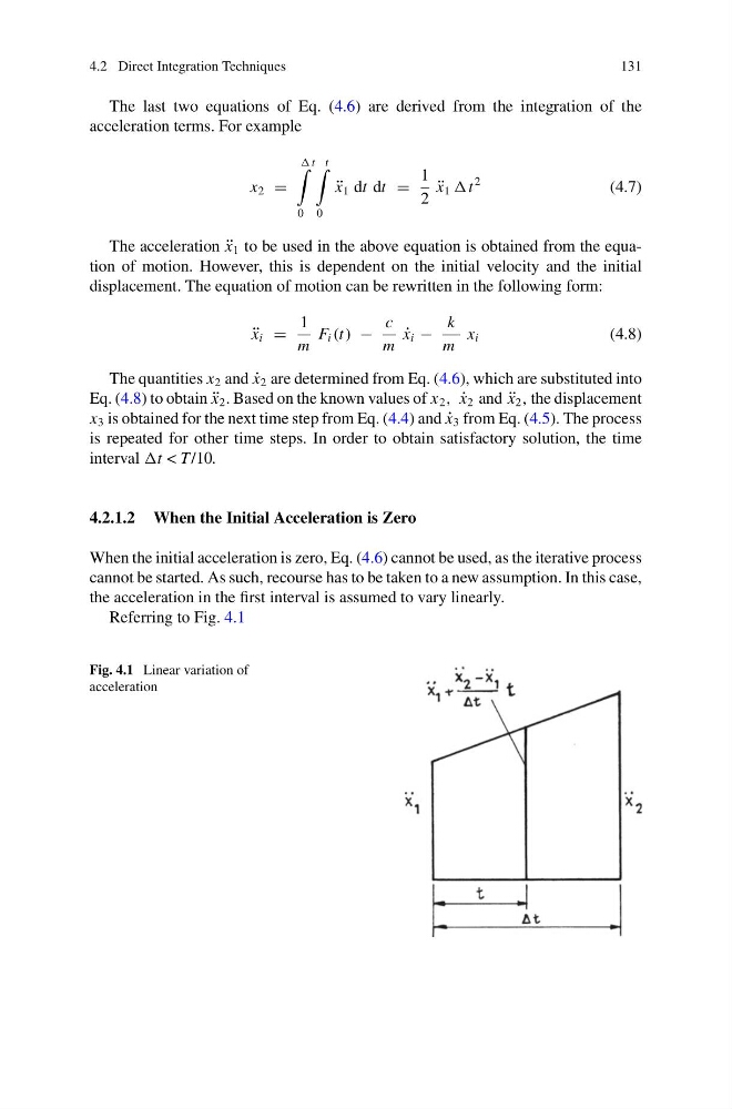
the acceleration in the first interval is assumed to vary linearly.
Referring to Fig. 4.1
Fig. 4.1 Linear variation of
acceleration
131
The last two equations of Eq. (4.6) are derived from the integration of the
acceleration terms. For example
x 2 =
t
0
t
0
¨
x 1 dt dt =
1
2
¨
x 1 t
2
(4.7)
The acceleration ¨
x 1 to be used in the above equation is obtained from the equation of motion. However, this is dependent on the initial velocity and the initial
displacement. The equation of motion can be rewritten in the following form:
¨
x i =
1
m
F i (t) −
c
m
˙
x i −
k
m
x i
(4.8)
The quantities x 2 and ˙
x 2 are determined from Eq. (4.6), which are substituted into
Eq. (4.8) to obtain ¨
x 2 . Based on the known values of x 2 , ˙
x 2 and ¨
x 2 , the displacement
x 3 is obtained for the next time step from Eq. (4.4) and ˙
x 3 from Eq. (4.5). The process
is repeated for other time steps. In order to obtain satisfactory solution, the time
interval t < T /10.
4.2.1.2 When the Initial Acceleration is Zero
When the initial acceleration is zero, Eq. (4.6) cannot be used, as the iterative process
cannot be started. As such, recourse has to be taken to a new assumption. In this case,
the acceleration in the first interval is assumed to vary linearly.
Referring to Fig. 4.1
Fig. 4.1 Linear variation of
acceleration