

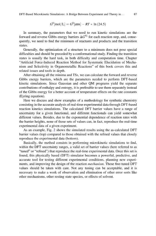
G
0 mol=L
½
¼G
0 atm
½ ÀRT Ã ln 24:5
ð
Þ
In summary, the parameters that we need to run kinetic simulations are the
forward and reverse Gibbs energy barriers ΔG
0{ for each reaction step, and, consequently, we need to find the minimum of reactants and products and the transition
states.
Generally, the optimization of a structure to a minimum does not pose special
difficulties and should be preceded by a conformational study. Finding the transition
states is usually the hard task, in both difficulty and computation time. Chapter
“Artificial Force-Induced Reaction Method for Systematic Elucidation of Mechanism and Selectivity in Organometallic Reactions” of this book covers this and
related issues and tools in depth.
After obtaining all the minima and TSs, we can calculate the forward and reverse
Gibbs energy barriers, which are the parameters needed to perform DFT-based
kinetic simulations. Since Gaussian and other QM programs yield the separate
contributions of enthalpy and entropy, it is preferable to use them separately instead
of the Gibbs energy for a better account of temperature effects on the rate constants
(Eyring equation).
Here we discuss and show examples of a methodology for synthetic chemistry
consisting in the accurate analysis of real-time experimental data through DFT-based
reaction kinetics simulations. The calculated DFT barrier values have a range of
uncertainty for a given functional, and different functionals can yield somewhat
different values. Besides, due to the exponential dependence of reaction rates with
the barrier heights, none of those sets of values can, in fact, reproduce the real-time
experimental data of a given experiment.
As an example, Fig. 2 shows the simulated results using the as-calculated DFT
barrier values (top) compared to those obtained with the refined values that closely
reproduce the experimental data (bottom).
Basically, the method consists in performing microkinetic simulations to find,
within the DFT uncertainty ranges, a valid set of barrier values (here referred to as
“tuned” or “refined”) that reproduce the real-time experimental data. Once this set is
found, this physically based (DFT) simulator becomes a powerful, predictive, and
accurate tool for testing different experimental conditions, planning new experiments, and improving the design of the reaction mechanism. Those fine-tuned DFT
values should be taken with care. Not any tuning can be acceptable, and it is
necessary to make a work of observation and elimination of other error sorts like
other mechanisms, other resting state species, or effects of solvent.
DFT-Based Microkinetic Simulations: A Bridge Between Experiment and Theory in. . .
87
0 mol=L
½
¼G
0 atm
½ ÀRT Ã ln 24:5
ð
Þ
In summary, the parameters that we need to run kinetic simulations are the
forward and reverse Gibbs energy barriers ΔG
0{ for each reaction step, and, consequently, we need to find the minimum of reactants and products and the transition
states.
Generally, the optimization of a structure to a minimum does not pose special
difficulties and should be preceded by a conformational study. Finding the transition
states is usually the hard task, in both difficulty and computation time. Chapter
“Artificial Force-Induced Reaction Method for Systematic Elucidation of Mechanism and Selectivity in Organometallic Reactions” of this book covers this and
related issues and tools in depth.
After obtaining all the minima and TSs, we can calculate the forward and reverse
Gibbs energy barriers, which are the parameters needed to perform DFT-based
kinetic simulations. Since Gaussian and other QM programs yield the separate
contributions of enthalpy and entropy, it is preferable to use them separately instead
of the Gibbs energy for a better account of temperature effects on the rate constants
(Eyring equation).
Here we discuss and show examples of a methodology for synthetic chemistry
consisting in the accurate analysis of real-time experimental data through DFT-based
reaction kinetics simulations. The calculated DFT barrier values have a range of
uncertainty for a given functional, and different functionals can yield somewhat
different values. Besides, due to the exponential dependence of reaction rates with
the barrier heights, none of those sets of values can, in fact, reproduce the real-time
experimental data of a given experiment.
As an example, Fig. 2 shows the simulated results using the as-calculated DFT
barrier values (top) compared to those obtained with the refined values that closely
reproduce the experimental data (bottom).
Basically, the method consists in performing microkinetic simulations to find,
within the DFT uncertainty ranges, a valid set of barrier values (here referred to as
“tuned” or “refined”) that reproduce the real-time experimental data. Once this set is
found, this physically based (DFT) simulator becomes a powerful, predictive, and
accurate tool for testing different experimental conditions, planning new experiments, and improving the design of the reaction mechanism. Those fine-tuned DFT
values should be taken with care. Not any tuning can be acceptable, and it is
necessary to make a work of observation and elimination of other error sorts like
other mechanisms, other resting state species, or effects of solvent.
DFT-Based Microkinetic Simulations: A Bridge Between Experiment and Theory in. . .
87