

5 The Theoretical Model
Once an appropriate model of the chemical system has been designed, the next step
is the choice of the computational methodology (the theoretical model) to obtain an
“accurate” energy of the computed system. It is important to remember that quantum
mechanical calculations afford the internal energy of the system (electronic + nuclear
at fixed nuclei positions) in vacuum and at 0 K. However, the reactions one needs to
simulate take place usually in solution at temperatures between 298 and 398 K.
Moreover, one needs to compute Gibbs energies because equilibrium and rate
constants depend on differences in Gibbs energies, not on internal energies. The
transformation of the internal energies into the Gibbs energies in solution (G sol ) adds
additional approximations to those already inherent to the internal energies. The
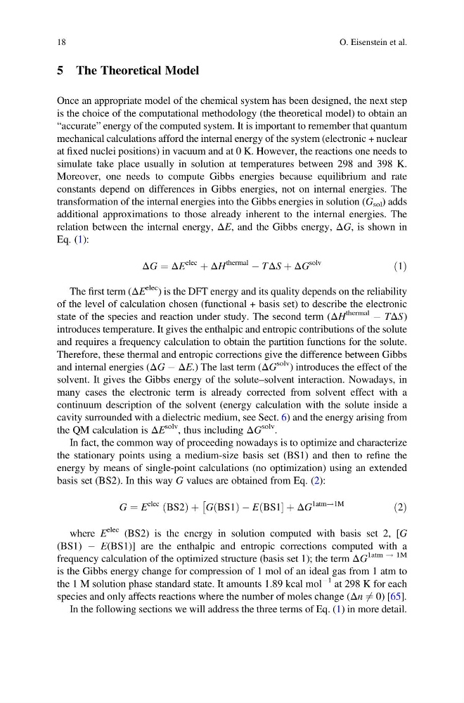
relation between the internal energy, ΔE, and the Gibbs energy, ΔG, is shown in
Eq. (1):
ΔG ¼ ΔE
elec
þ ΔH
thermal
À TΔS þ ΔG
solv
ð1Þ
The first term (ΔE
elec ) is the DFT energy and its quality depends on the reliability
of the level of calculation chosen (functional + basis set) to describe the electronic
state of the species and reaction under study. The second term (ΔH
thermal
À TΔS)
introduces temperature. It gives the enthalpic and entropic contributions of the solute
and requires a frequency calculation to obtain the partition functions for the solute.
Therefore, these thermal and entropic corrections give the difference between Gibbs
and internal energies (ΔG À ΔE.) The last term (ΔG
solv
) introduces the effect of the
solvent. It gives the Gibbs energy of the solute–solvent interaction. Nowadays, in
many cases the electronic term is already corrected from solvent effect with a
continuum description of the solvent (energy calculation with the solute inside a
cavity surrounded with a dielectric medium, see Sect. 6) and the energy arising from
the QM calculation is ΔE
solv , thus including ΔG
solv
.
In fact, the common way of proceeding nowadays is to optimize and characterize
the stationary points using a medium-size basis set (BS1) and then to refine the
energy by means of single-point calculations (no optimization) using an extended
basis set (BS2). In this way G values are obtained from Eq. (2):
G ¼ E
elec BS2
ð
Þþ G BS1
ð
ÞÀE BS1
ð
þΔG
1atm!1M
Â
ð2Þ
where E
elec (BS2) is the energy in solution computed with basis set 2, [G
(BS1) À E(BS1)] are the enthalpic and entropic corrections computed with a
frequency calculation of the optimized structure (basis set 1); the term ΔG
1atm ! 1M
is the Gibbs energy change for compression of 1 mol of an ideal gas from 1 atm to
the 1 M solution phase standard state. It amounts 1.89 kcal mol
À1 at 298 K for each
species and only affects reactions where the number of moles change (Δn 6 ¼ 0) [65].
In the following sections we will address the three terms of Eq. (1) in more detail.
18
O. Eisenstein et al.
Once an appropriate model of the chemical system has been designed, the next step
is the choice of the computational methodology (the theoretical model) to obtain an
“accurate” energy of the computed system. It is important to remember that quantum
mechanical calculations afford the internal energy of the system (electronic + nuclear
at fixed nuclei positions) in vacuum and at 0 K. However, the reactions one needs to
simulate take place usually in solution at temperatures between 298 and 398 K.
Moreover, one needs to compute Gibbs energies because equilibrium and rate
constants depend on differences in Gibbs energies, not on internal energies. The
transformation of the internal energies into the Gibbs energies in solution (G sol ) adds
additional approximations to those already inherent to the internal energies. The
relation between the internal energy, ΔE, and the Gibbs energy, ΔG, is shown in
Eq. (1):
ΔG ¼ ΔE
elec
þ ΔH
thermal
À TΔS þ ΔG
solv
ð1Þ
The first term (ΔE
elec ) is the DFT energy and its quality depends on the reliability
of the level of calculation chosen (functional + basis set) to describe the electronic
state of the species and reaction under study. The second term (ΔH
thermal
À TΔS)
introduces temperature. It gives the enthalpic and entropic contributions of the solute
and requires a frequency calculation to obtain the partition functions for the solute.
Therefore, these thermal and entropic corrections give the difference between Gibbs
and internal energies (ΔG À ΔE.) The last term (ΔG
solv
) introduces the effect of the
solvent. It gives the Gibbs energy of the solute–solvent interaction. Nowadays, in
many cases the electronic term is already corrected from solvent effect with a
continuum description of the solvent (energy calculation with the solute inside a
cavity surrounded with a dielectric medium, see Sect. 6) and the energy arising from
the QM calculation is ΔE
solv , thus including ΔG
solv
.
In fact, the common way of proceeding nowadays is to optimize and characterize
the stationary points using a medium-size basis set (BS1) and then to refine the
energy by means of single-point calculations (no optimization) using an extended
basis set (BS2). In this way G values are obtained from Eq. (2):
G ¼ E
elec BS2
ð
Þþ G BS1
ð
ÞÀE BS1
ð
þΔG
1atm!1M
Â
ð2Þ
where E
elec (BS2) is the energy in solution computed with basis set 2, [G
(BS1) À E(BS1)] are the enthalpic and entropic corrections computed with a
frequency calculation of the optimized structure (basis set 1); the term ΔG
1atm ! 1M
is the Gibbs energy change for compression of 1 mol of an ideal gas from 1 atm to
the 1 M solution phase standard state. It amounts 1.89 kcal mol
À1 at 298 K for each
species and only affects reactions where the number of moles change (Δn 6 ¼ 0) [65].
In the following sections we will address the three terms of Eq. (1) in more detail.
18
O. Eisenstein et al.