

88
13 Non-Fock Representations
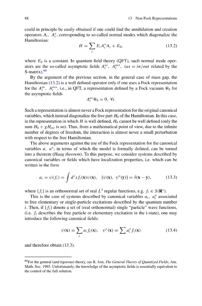
could in principle be easily obtained if one could find the annihilation and creation
operators A i , A
∗
i , corresponding to so-called normal modes which diagonalize the
Hamiltonian:
H =
i
E i A
∗
i A i + E 0 ,
(13.2)
where E 0 is a constant. In quantum field theory (QFT), such normal mode operators are the so-called asymptotic fields A
as
i , A
as∗
i , (as = in/out related by the
S-matrix).
60
By the argument of the previous section, in the general case of mass gap, the
Hamiltonian (13.2) is a well defined operator only if one uses a Fock representation
for the A
as
i , A
as∗
i , i.e., in QFT, a representation defined by a Fock vacuum 0 for
the asymptotic fields
A
as
i 0 = 0, ∀i.
Such a representation is almost never a Fock representation for the original canonical
variables, which instead diagonalize the free part H 0 of the Hamiltonian. In this case,
in the representation in which H is well defined, H 0 cannot be well defined (only the
sum H 0 + g H int is so). Thus, from a mathematical point of view, due to the infinite
number of degrees of freedom, the interaction is almost never a small perturbation
with respect to the free Hamiltonian.
The above arguments against the use of the Fock representation for the canonical
variables a, a
∗ , in terms of which the model is formally defined, can be turned
into a theorem (Haag theorem). To this purpose, we consider systems described by
canonical variables or fields which have localization properties, i.e. which can be
written in the form
a i = ψ( f i ) =
d
s x f i (x)ψ(x), [ψ(x), ψ
∗
(y)] = δ(x − y),
(13.3)
where { f i } is an orthonormal set of real L
2 regular functions, e.g. f i ∈ S(R
s
).
This is the case of systems described by canonical variables a i , a
∗
i associated
to free elementary or single-particle excitations described by the quantum number
i. Then, if { f i } denote a set of (real orthonormal) single “particle” wave functions,
(i.e. f i describes the free particle or elementary excitation in the i-state), one may
introduce the following canonical fields:
ψ(x) ≡
i
a i f i (x), ψ
∗
(x) ≡
a
∗
i f i (x)
(13.4)
and therefore obtain (13.3).
60 For the general (and rigorous) theory, see R. Jost, The General Theory of Quantized Fields, Am.
Math. Soc. 1965. Unfortunately, the knowledge of the asymptotic fields is essentially equivalent to
the control of the full solution.
13 Non-Fock Representations
could in principle be easily obtained if one could find the annihilation and creation
operators A i , A
∗
i , corresponding to so-called normal modes which diagonalize the
Hamiltonian:
H =
i
E i A
∗
i A i + E 0 ,
(13.2)
where E 0 is a constant. In quantum field theory (QFT), such normal mode operators are the so-called asymptotic fields A
as
i , A
as∗
i , (as = in/out related by the
S-matrix).
60
By the argument of the previous section, in the general case of mass gap, the
Hamiltonian (13.2) is a well defined operator only if one uses a Fock representation
for the A
as
i , A
as∗
i , i.e., in QFT, a representation defined by a Fock vacuum 0 for
the asymptotic fields
A
as
i 0 = 0, ∀i.
Such a representation is almost never a Fock representation for the original canonical
variables, which instead diagonalize the free part H 0 of the Hamiltonian. In this case,
in the representation in which H is well defined, H 0 cannot be well defined (only the
sum H 0 + g H int is so). Thus, from a mathematical point of view, due to the infinite
number of degrees of freedom, the interaction is almost never a small perturbation
with respect to the free Hamiltonian.
The above arguments against the use of the Fock representation for the canonical
variables a, a
∗ , in terms of which the model is formally defined, can be turned
into a theorem (Haag theorem). To this purpose, we consider systems described by
canonical variables or fields which have localization properties, i.e. which can be
written in the form
a i = ψ( f i ) =
d
s x f i (x)ψ(x), [ψ(x), ψ
∗
(y)] = δ(x − y),
(13.3)
where { f i } is an orthonormal set of real L
2 regular functions, e.g. f i ∈ S(R
s
).
This is the case of systems described by canonical variables a i , a
∗
i associated
to free elementary or single-particle excitations described by the quantum number
i. Then, if { f i } denote a set of (real orthonormal) single “particle” wave functions,
(i.e. f i describes the free particle or elementary excitation in the i-state), one may
introduce the following canonical fields:
ψ(x) ≡
i
a i f i (x), ψ
∗
(x) ≡
a
∗
i f i (x)
(13.4)
and therefore obtain (13.3).
60 For the general (and rigorous) theory, see R. Jost, The General Theory of Quantized Fields, Am.
Math. Soc. 1965. Unfortunately, the knowledge of the asymptotic fields is essentially equivalent to
the control of the full solution.