

8 Examples
43
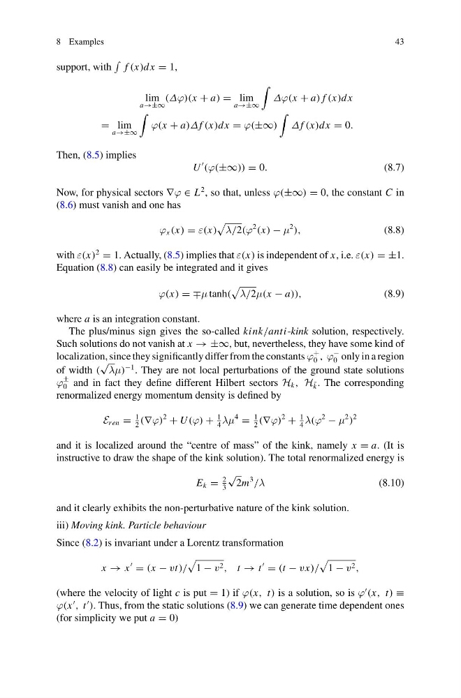
support, with
f (x)dx = 1,
lim
a→±∞
(Δϕ)(x + a) = lim
a→±∞
Δϕ(x + a) f (x)dx
= lim
a→±∞
ϕ(x + a)Δf (x)dx = ϕ(±∞)
Δf (x)dx = 0.
Then, (8.5) implies
U
(ϕ(±∞)) = 0.
(8.7)
Now, for physical sectors ∇ϕ ∈ L
2 , so that, unless ϕ(±∞) = 0, the constant C in
(8.6) must vanish and one has
ϕ x (x) = ε(x)
λ/2(ϕ
2
(x) − μ
2
),
(8.8)
with ε(x)
2
= 1. Actually, (8.5) implies that ε(x) is independent of x, i.e. ε(x) = ±1.
Equation (8.8) can easily be integrated and it gives
ϕ(x) = ∓μ tanh(
λ/2μ(x − a)),
(8.9)
where a is an integration constant.
The plus/minus sign gives the so-called kink/anti-kink solution, respectively.
Such solutions do not vanish at x → ±∞, but, nevertheless, they have some kind of
localization, since they significantly differ from the constants ϕ
+
0 , ϕ
−
0 only in a region
of width (
√ λμ)
−1 . They are not local perturbations of the ground state solutions
ϕ
±
0 and in fact they define different Hilbert sectors H k , H¯ k . The corresponding
renormalized energy momentum density is defined by
E ren =
1
2
(∇ϕ)
2
+ U (ϕ) +
1
4
λμ
4
=
1
2
(∇ϕ)
2
+
1
4
λ(ϕ
2
− μ
2
)
2
and it is localized around the “centre of mass” of the kink, namely x = a. (It is
instructive to draw the shape of the kink solution). The total renormalized energy is
E k =
2
3
√
2m
3
/λ
(8.10)
and it clearly exhibits the non-perturbative nature of the kink solution.
iii) Moving kink. Particle behaviour
Since (8.2) is invariant under a Lorentz transformation
x → x
= (x − vt)/
1 − v 2 , t → t
= (t − vx)/
1 − v 2 ,
(where the velocity of light c is put = 1) if ϕ(x, t) is a solution, so is ϕ
(x, t) ≡
ϕ(x
, t
). Thus, from the static solutions (8.9) we can generate time dependent ones
(for simplicity we put a = 0)
43
support, with
f (x)dx = 1,
lim
a→±∞
(Δϕ)(x + a) = lim
a→±∞
Δϕ(x + a) f (x)dx
= lim
a→±∞
ϕ(x + a)Δf (x)dx = ϕ(±∞)
Δf (x)dx = 0.
Then, (8.5) implies
U
(ϕ(±∞)) = 0.
(8.7)
Now, for physical sectors ∇ϕ ∈ L
2 , so that, unless ϕ(±∞) = 0, the constant C in
(8.6) must vanish and one has
ϕ x (x) = ε(x)
λ/2(ϕ
2
(x) − μ
2
),
(8.8)
with ε(x)
2
= 1. Actually, (8.5) implies that ε(x) is independent of x, i.e. ε(x) = ±1.
Equation (8.8) can easily be integrated and it gives
ϕ(x) = ∓μ tanh(
λ/2μ(x − a)),
(8.9)
where a is an integration constant.
The plus/minus sign gives the so-called kink/anti-kink solution, respectively.
Such solutions do not vanish at x → ±∞, but, nevertheless, they have some kind of
localization, since they significantly differ from the constants ϕ
+
0 , ϕ
−
0 only in a region
of width (
√ λμ)
−1 . They are not local perturbations of the ground state solutions
ϕ
±
0 and in fact they define different Hilbert sectors H k , H¯ k . The corresponding
renormalized energy momentum density is defined by
E ren =
1
2
(∇ϕ)
2
+ U (ϕ) +
1
4
λμ
4
=
1
2
(∇ϕ)
2
+
1
4
λ(ϕ
2
− μ
2
)
2
and it is localized around the “centre of mass” of the kink, namely x = a. (It is
instructive to draw the shape of the kink solution). The total renormalized energy is
E k =
2
3
√
2m
3
/λ
(8.10)
and it clearly exhibits the non-perturbative nature of the kink solution.
iii) Moving kink. Particle behaviour
Since (8.2) is invariant under a Lorentz transformation
x → x
= (x − vt)/
1 − v 2 , t → t
= (t − vx)/
1 − v 2 ,
(where the velocity of light c is put = 1) if ϕ(x, t) is a solution, so is ϕ
(x, t) ≡
ϕ(x
, t
). Thus, from the static solutions (8.9) we can generate time dependent ones
(for simplicity we put a = 0)