

18
4 General Properties of Solutions of Classical Field Equations
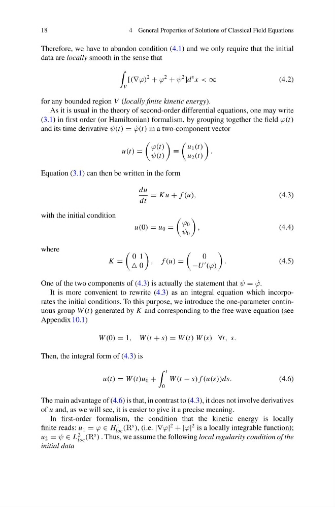
Therefore, we have to abandon condition (4.1) and we only require that the initial
data are locally smooth in the sense that
V
[(∇ϕ)
2
+ ϕ
2
+ ψ
2
]d
s x < ∞
(4.2)
for any bounded region V (locally finite kinetic energy).
As it is usual in the theory of second-order differential equations, one may write
(3.1) in first order (or Hamiltonian) formalism, by grouping together the field ϕ(t)
and its time derivative ψ(t) = ˙
ϕ(t) in a two-component vector
u(t) =
ϕ(t)
ψ(t)
≡
u 1 (t)
u 2 (t)
.
Equation (3.1) can then be written in the form
du
dt
= K u + f (u),
(4.3)
with the initial condition
u(0) = u 0 =
ϕ 0
ψ 0
,
(4.4)
where
K =
0 1
0
, f (u) =
0
−U
(ϕ)
.
(4.5)
One of the two components of (4.3) is actually the statement that ψ = ˙
ϕ.
It is more convenient to rewrite (4.3) as an integral equation which incorporates the initial conditions. To this purpose, we introduce the one-parameter continuous group W (t) generated by K and corresponding to the free wave equation (see
Appendix 10.1)
W (0) = 1, W (t + s) = W (t) W (s) ∀t, s.
Then, the integral form of (4.3) is
u(t) = W (t)u 0 +
t
0
W (t − s) f (u(s))ds.
(4.6)
The main advantage of (4.6) is that, in contrast to (4.3), it does not involve derivatives
of u and, as we will see, it is easier to give it a precise meaning.
In first-order formalism, the condition that the kinetic energy is locally
finite reads: u 1 = ϕ ∈ H
1
loc (R
s
), (i.e. |∇ϕ|
2
+ |ϕ|
2 is a locally integrable function);
u 2 = ψ ∈ L
2
loc (R
s
) . Thus, we assume the following local regularity condition of the
initial data
4 General Properties of Solutions of Classical Field Equations
Therefore, we have to abandon condition (4.1) and we only require that the initial
data are locally smooth in the sense that
V
[(∇ϕ)
2
+ ϕ
2
+ ψ
2
]d
s x < ∞
(4.2)
for any bounded region V (locally finite kinetic energy).
As it is usual in the theory of second-order differential equations, one may write
(3.1) in first order (or Hamiltonian) formalism, by grouping together the field ϕ(t)
and its time derivative ψ(t) = ˙
ϕ(t) in a two-component vector
u(t) =
ϕ(t)
ψ(t)
≡
u 1 (t)
u 2 (t)
.
Equation (3.1) can then be written in the form
du
dt
= K u + f (u),
(4.3)
with the initial condition
u(0) = u 0 =
ϕ 0
ψ 0
,
(4.4)
where
K =
0 1
0
, f (u) =
0
−U
(ϕ)
.
(4.5)
One of the two components of (4.3) is actually the statement that ψ = ˙
ϕ.
It is more convenient to rewrite (4.3) as an integral equation which incorporates the initial conditions. To this purpose, we introduce the one-parameter continuous group W (t) generated by K and corresponding to the free wave equation (see
Appendix 10.1)
W (0) = 1, W (t + s) = W (t) W (s) ∀t, s.
Then, the integral form of (4.3) is
u(t) = W (t)u 0 +
t
0
W (t − s) f (u(s))ds.
(4.6)
The main advantage of (4.6) is that, in contrast to (4.3), it does not involve derivatives
of u and, as we will see, it is easier to give it a precise meaning.
In first-order formalism, the condition that the kinetic energy is locally
finite reads: u 1 = ϕ ∈ H
1
loc (R
s
), (i.e. |∇ϕ|
2
+ |ϕ|
2 is a locally integrable function);
u 2 = ψ ∈ L
2
loc (R
s
) . Thus, we assume the following local regularity condition of the
initial data