

23.4 Bose–Einstein Condensation and Symmetry Breaking
165
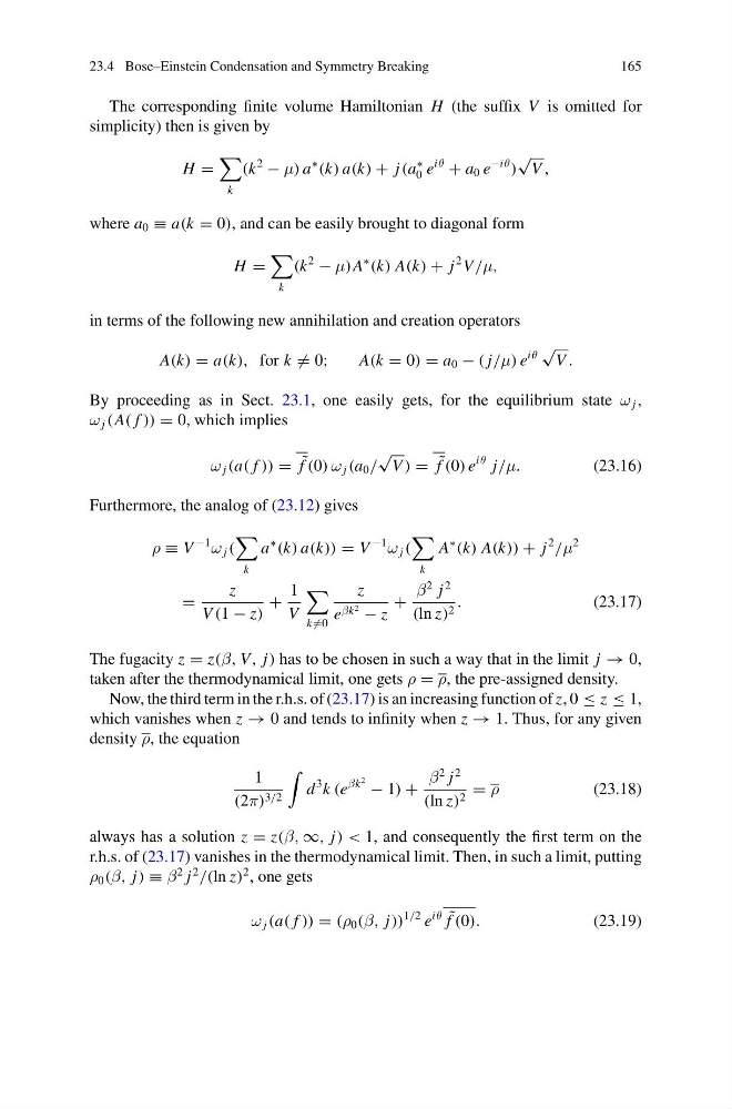
The corresponding finite volume Hamiltonian H (the suffix V is omitted for
simplicity) then is given by
H =
k
(k
2
− μ) a
∗
(k) a(k) + j (a
∗
0 e
iθ
+ a 0 e
−iθ
)
√
V ,
where a 0 ≡ a(k = 0), and can be easily brought to diagonal form
H =
k
(k
2
− μ)A
∗
(k) A(k) + j
2 V /μ,
in terms of the following new annihilation and creation operators
A(k) = a(k), for k = 0;
A(k = 0) = a 0 − ( j/μ) e
iθ
√
V .
By proceeding as in Sect. 23.1, one easily gets, for the equilibrium state ω j ,
ω j (A( f )) = 0, which implies
ω j (a( f )) = ˜
f (0) ω j (a 0 /
√
V ) = ˜
f (0) e
iθ j/μ.
(23.16)
Furthermore, the analog of (23.12) gives
ρ ≡ V
−1
ω j (
k
a
∗
(k) a(k)) = V
−1
ω j (
k
A
∗
(k) A(k)) + j
2
/μ
2
=
z
V (1 − z)
+
1
V
k =0
z
e βk 2 − z
+
β
2 j
2
(ln z) 2 .
(23.17)
The fugacity z = z(β, V, j) has to be chosen in such a way that in the limit j → 0,
taken after the thermodynamical limit, one gets ρ = ρ, the pre-assigned density.
Now, the third term in the r.h.s. of (23.17) is an increasing function of z, 0 ≤ z ≤ 1,
which vanishes when z → 0 and tends to infinity when z → 1. Thus, for any given
density ρ, the equation
1
(2π) 3/2
d
3 k (e
βk
2 − 1) +
β
2 j
2
(ln z) 2 = ρ
(23.18)
always has a solution z = z(β, ∞, j) < 1, and consequently the first term on the
r.h.s. of (23.17) vanishes in the thermodynamical limit. Then, in such a limit, putting
ρ 0 (β, j) ≡ β
2 j
2
/(ln z)
2 , one gets
ω j (a( f )) = (ρ 0 (β, j))
1/2 e
iθ ˜
f (0).
(23.19)
165
The corresponding finite volume Hamiltonian H (the suffix V is omitted for
simplicity) then is given by
H =
k
(k
2
− μ) a
∗
(k) a(k) + j (a
∗
0 e
iθ
+ a 0 e
−iθ
)
√
V ,
where a 0 ≡ a(k = 0), and can be easily brought to diagonal form
H =
k
(k
2
− μ)A
∗
(k) A(k) + j
2 V /μ,
in terms of the following new annihilation and creation operators
A(k) = a(k), for k = 0;
A(k = 0) = a 0 − ( j/μ) e
iθ
√
V .
By proceeding as in Sect. 23.1, one easily gets, for the equilibrium state ω j ,
ω j (A( f )) = 0, which implies
ω j (a( f )) = ˜
f (0) ω j (a 0 /
√
V ) = ˜
f (0) e
iθ j/μ.
(23.16)
Furthermore, the analog of (23.12) gives
ρ ≡ V
−1
ω j (
k
a
∗
(k) a(k)) = V
−1
ω j (
k
A
∗
(k) A(k)) + j
2
/μ
2
=
z
V (1 − z)
+
1
V
k =0
z
e βk 2 − z
+
β
2 j
2
(ln z) 2 .
(23.17)
The fugacity z = z(β, V, j) has to be chosen in such a way that in the limit j → 0,
taken after the thermodynamical limit, one gets ρ = ρ, the pre-assigned density.
Now, the third term in the r.h.s. of (23.17) is an increasing function of z, 0 ≤ z ≤ 1,
which vanishes when z → 0 and tends to infinity when z → 1. Thus, for any given
density ρ, the equation
1
(2π) 3/2
d
3 k (e
βk
2 − 1) +
β
2 j
2
(ln z) 2 = ρ
(23.18)
always has a solution z = z(β, ∞, j) < 1, and consequently the first term on the
r.h.s. of (23.17) vanishes in the thermodynamical limit. Then, in such a limit, putting
ρ 0 (β, j) ≡ β
2 j
2
/(ln z)
2 , one gets
ω j (a( f )) = (ρ 0 (β, j))
1/2 e
iθ ˜
f (0).
(23.19)