

150
22 ∗ Thermal States
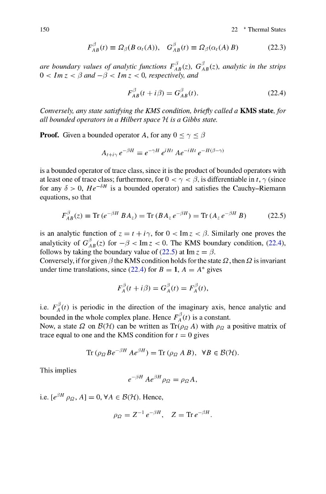
F
β
AB (t) ≡ Ω β (B α t (A)), G
β
AB (t) ≡ Ω β (α t (A) B)
(22.3)
are boundary values of analytic functions F
β
AB (z), G
β
AB (z), analytic in the strips
0 < I m z < β and −β < I m z < 0, respectively, and
F
β
AB (t + iβ) = G
β
AB (t).
(22.4)
Conversely, any state satisfying the KMS condition, briefly called a KMS state, for
all bounded operators in a Hilbert space H is a Gibbs state.
Proof. Given a bounded operator A, for any 0 ≤ γ ≤ β
A t+iγ e
−β H
≡ e
−γ H e
i Ht Ae
−i Ht e
−H (β−γ)
is a bounded operator of trace class, since it is the product of bounded operators with
at least one of trace class; furthermore, for 0 < γ < β, is differentiable in t, γ (since
for any δ > 0, He
−δ H is a bounded operator) and satisfies the Cauchy–Riemann
equations, so that
F
β
AB (z) ≡ Tr (e
−β H B A z ) = Tr (B A z e
−β H
) = Tr (A z e
−β H B)
(22.5)
is an analytic function of z = t + iγ, for 0 < Im z < β. Similarly one proves the
analyticity of G
β
AB (z) for −β < Im z < 0. The KMS boundary condition, (22.4),
follows by taking the boundary value of (22.5) at Im z = β.
Conversely, if for given β the KMS condition holds for the state Ω, then Ω is invariant
under time translations, since (22.4) for B = 1, A = A
∗ gives
F
β
A (t + iβ) = G
β
A (t) = F
β
A (t),
i.e. F
β
A (t) is periodic in the direction of the imaginary axis, hence analytic and
bounded in the whole complex plane. Hence F
β
A (t) is a constant.
Now, a state Ω on B(H) can be written as Tr(ρ Ω A) with ρ Ω a positive matrix of
trace equal to one and the KMS condition for t = 0 gives
Tr (ρ Ω Be
−β H Ae
β H
) = Tr (ρ Ω A B), ∀B ∈ B(H).
This implies
e
−β H Ae
β H
ρ Ω = ρ Ω A,
i.e. [e
β H
ρ Ω , A] = 0, ∀A ∈ B(H). Hence,
ρ Ω = Z
−1 e
−β H
, Z = Tr e
−β H
.
22 ∗ Thermal States
F
β
AB (t) ≡ Ω β (B α t (A)), G
β
AB (t) ≡ Ω β (α t (A) B)
(22.3)
are boundary values of analytic functions F
β
AB (z), G
β
AB (z), analytic in the strips
0 < I m z < β and −β < I m z < 0, respectively, and
F
β
AB (t + iβ) = G
β
AB (t).
(22.4)
Conversely, any state satisfying the KMS condition, briefly called a KMS state, for
all bounded operators in a Hilbert space H is a Gibbs state.
Proof. Given a bounded operator A, for any 0 ≤ γ ≤ β
A t+iγ e
−β H
≡ e
−γ H e
i Ht Ae
−i Ht e
−H (β−γ)
is a bounded operator of trace class, since it is the product of bounded operators with
at least one of trace class; furthermore, for 0 < γ < β, is differentiable in t, γ (since
for any δ > 0, He
−δ H is a bounded operator) and satisfies the Cauchy–Riemann
equations, so that
F
β
AB (z) ≡ Tr (e
−β H B A z ) = Tr (B A z e
−β H
) = Tr (A z e
−β H B)
(22.5)
is an analytic function of z = t + iγ, for 0 < Im z < β. Similarly one proves the
analyticity of G
β
AB (z) for −β < Im z < 0. The KMS boundary condition, (22.4),
follows by taking the boundary value of (22.5) at Im z = β.
Conversely, if for given β the KMS condition holds for the state Ω, then Ω is invariant
under time translations, since (22.4) for B = 1, A = A
∗ gives
F
β
A (t + iβ) = G
β
A (t) = F
β
A (t),
i.e. F
β
A (t) is periodic in the direction of the imaginary axis, hence analytic and
bounded in the whole complex plane. Hence F
β
A (t) is a constant.
Now, a state Ω on B(H) can be written as Tr(ρ Ω A) with ρ Ω a positive matrix of
trace equal to one and the KMS condition for t = 0 gives
Tr (ρ Ω Be
−β H Ae
β H
) = Tr (ρ Ω A B), ∀B ∈ B(H).
This implies
e
−β H Ae
β H
ρ Ω = ρ Ω A,
i.e. [e
β H
ρ Ω , A] = 0, ∀A ∈ B(H). Hence,
ρ Ω = Z
−1 e
−β H
, Z = Tr e
−β H
.