

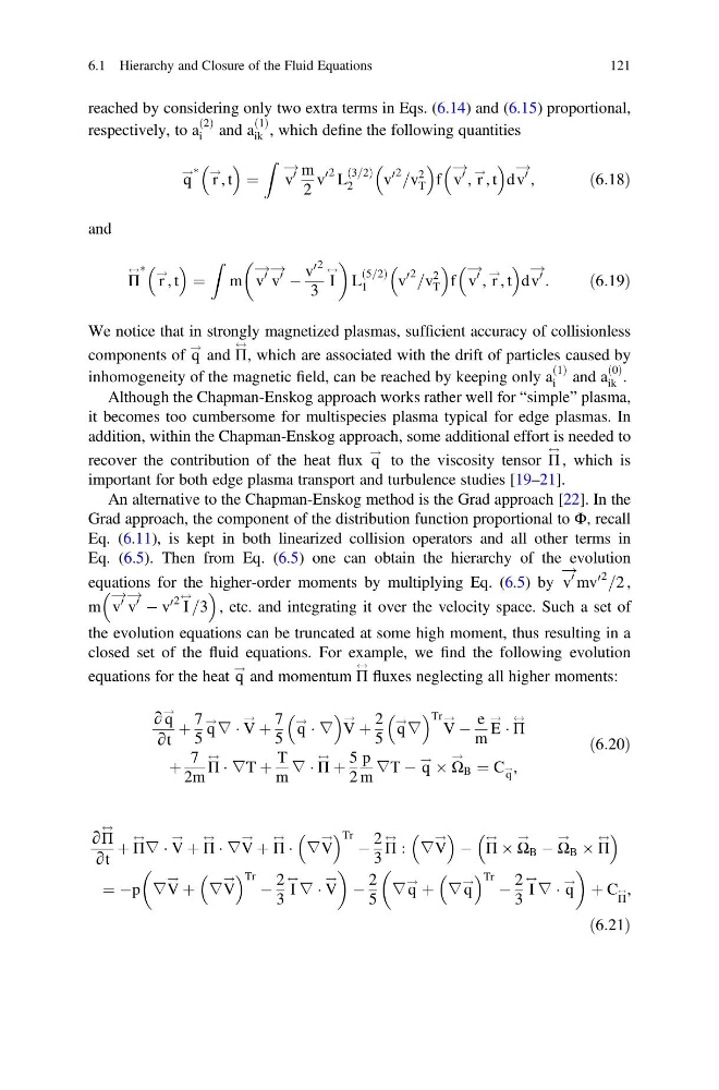
reached by considering only two extra terms in Eqs. (6.14) and (6.15) proportional,
respectively, to a
2
ð Þ
i and a
1
ð Þ
ik , which define the following quantities
q
! Ã
r
!
, t
¼
Z
v
0
! m
2
v
0 2 L
3=2
ð
Þ
2
v
0 2 =v
2
T
f v
0
!
, r
! , t
d v
0
!
,
ð6:18Þ
and
Π
$ Ã
r
!
, t
¼
Z
m v
0
!
v
0
! À
v
0 2
3
I
$
L
5=2
ð
Þ
1
v
0 2 =v
2
T
f v
0
!
, r
!
, t
dv
0
!
:
ð6:19Þ
We notice that in strongly magnetized plasmas, sufficient accuracy of collisionless
components of q
! and Π
$
, which are associated with the drift of particles caused by
inhomogeneity of the magnetic field, can be reached by keeping only a
1
ð Þ
i and a
0
ð Þ
ik .
Although the Chapman-Enskog approach works rather well for “simple” plasma,
it becomes too cumbersome for multispecies plasma typical for edge plasmas. In
addition, within the Chapman-Enskog approach, some additional effort is needed to
recover the contribution of the heat flux q
! to the viscosity tensor Π
$
, which is
important for both edge plasma transport and turbulence studies [19–21].
An alternative to the Chapman-Enskog method is the Grad approach [22]. In the
Grad approach, the component of the distribution function proportional to Φ, recall
Eq. (6.11), is kept in both linearized collision operators and all other terms in
Eq. (6.5). Then from Eq. (6.5) one can obtain the hierarchy of the evolution
equations for the higher-order moments by multiplying Eq. (6.5) by v
0
!
mv
0 2 =2 ,
m v
0
!
v
0
! À v
0 2 I
$
=3
, etc. and integrating it over the velocity space. Such a set of
the evolution equations can be truncated at some high moment, thus resulting in a
closed set of the fluid equations. For example, we find the following evolution
equations for the heat q
! and momentum Π
$ fluxes neglecting all higher moments:
∂ q
!
∂t
þ
7
5
q
!
∇ Á V
! þ
7
5
q
! Á ∇
V
! þ
2
5
q
! ∇
Tr
V
! À
e
m
E
! Á Π
$
þ
7
2m
Π
$ Á ∇T þ
T
m
∇ Á Π
$ þ
5
2
p
m
∇T À q
! Â Ω
!
B ¼ C q
!,
ð6:20Þ
∂Π
$
∂t
þ Π
$ ∇ Á V
! þ Π
$ Á ∇V
! þ Π
$ Á ∇V
!
Tr À
2
3
Π
$ : ∇V
!
À Π
$ Â Ω
!
B À Ω
!
B Â Π
$
¼ Àp ∇V
! þ ∇V
!
Tr À
2
3
I
$ ∇ Á V
!
À
2
5
∇ q
! þ ∇ q
!
Tr À
2
3
I
$
∇ Á q
!
þ C Π
$ ,
ð6:21Þ
6.1 Hierarchy and Closure of the Fluid Equations
121
respectively, to a
2
ð Þ
i and a
1
ð Þ
ik , which define the following quantities
q
! Ã
r
!
, t
¼
Z
v
0
! m
2
v
0 2 L
3=2
ð
Þ
2
v
0 2 =v
2
T
f v
0
!
, r
! , t
d v
0
!
,
ð6:18Þ
and
Π
$ Ã
r
!
, t
¼
Z
m v
0
!
v
0
! À
v
0 2
3
I
$
L
5=2
ð
Þ
1
v
0 2 =v
2
T
f v
0
!
, r
!
, t
dv
0
!
:
ð6:19Þ
We notice that in strongly magnetized plasmas, sufficient accuracy of collisionless
components of q
! and Π
$
, which are associated with the drift of particles caused by
inhomogeneity of the magnetic field, can be reached by keeping only a
1
ð Þ
i and a
0
ð Þ
ik .
Although the Chapman-Enskog approach works rather well for “simple” plasma,
it becomes too cumbersome for multispecies plasma typical for edge plasmas. In
addition, within the Chapman-Enskog approach, some additional effort is needed to
recover the contribution of the heat flux q
! to the viscosity tensor Π
$
, which is
important for both edge plasma transport and turbulence studies [19–21].
An alternative to the Chapman-Enskog method is the Grad approach [22]. In the
Grad approach, the component of the distribution function proportional to Φ, recall
Eq. (6.11), is kept in both linearized collision operators and all other terms in
Eq. (6.5). Then from Eq. (6.5) one can obtain the hierarchy of the evolution
equations for the higher-order moments by multiplying Eq. (6.5) by v
0
!
mv
0 2 =2 ,
m v
0
!
v
0
! À v
0 2 I
$
=3
, etc. and integrating it over the velocity space. Such a set of
the evolution equations can be truncated at some high moment, thus resulting in a
closed set of the fluid equations. For example, we find the following evolution
equations for the heat q
! and momentum Π
$ fluxes neglecting all higher moments:
∂ q
!
∂t
þ
7
5
q
!
∇ Á V
! þ
7
5
q
! Á ∇
V
! þ
2
5
q
! ∇
Tr
V
! À
e
m
E
! Á Π
$
þ
7
2m
Π
$ Á ∇T þ
T
m
∇ Á Π
$ þ
5
2
p
m
∇T À q
! Â Ω
!
B ¼ C q
!,
ð6:20Þ
∂Π
$
∂t
þ Π
$ ∇ Á V
! þ Π
$ Á ∇V
! þ Π
$ Á ∇V
!
Tr À
2
3
Π
$ : ∇V
!
À Π
$ Â Ω
!
B À Ω
!
B Â Π
$
¼ Àp ∇V
! þ ∇V
!
Tr À
2
3
I
$ ∇ Á V
!
À
2
5
∇ q
! þ ∇ q
!
Tr À
2
3
I
$
∇ Á q
!
þ C Π
$ ,
ð6:21Þ
6.1 Hierarchy and Closure of the Fluid Equations
121