

16
2 The Nature of Light
where f v is the measured spectral flux density, the rate at which energy transfers
through a surface measured per second per unit area. In practice, AB and Vega are
almost identical, at least for objects with reasonably flat spectral energy distributions.
For the purposes of the practicals in this book, we will always use Vega magnitudes.
However, you should always note in your lab book which system you are referring
to.
Keep in mind that the flux you measure is the instrumental flux. This means that
when you apply Pogson’s formula or the various derivatives to that flux, what you
will get is an instrumental magnitude. If you wish to determine an actual physical magnitude, then you will need to undertake a much lengthier process, one that
accounts for the optics and the specific filter set that you are using.
Another subtlety concerns extended objects such as galaxies and nebulae. The
magnitude that is usually quoted for these is the integrated magnitude, which is the
total amount of light emitted by the object across the band in question. However,
this causes an observational difficulty. If you set your exposure time for such an
object based on its integrated magnitude, it will be underexposed, since the light is
spread out over more pixels than a star. A workaround for this difficulty is to use the
surface brightness, which is the magnitude per square arc second. (Effectively, this
is a magnitude density, if that makes sense.) The surface brightness has some issues
of its own in that it, too, has inbuilt assumptions—it treats objects as having even
brightness, when in fact, most of them will have concentrated brightness in one area
and more diffuse brightness elsewhere. It is best to keep in mind what sort of object
you are observing and to try to adjust your practice accordingly.
Later in this book we will discuss in depth the concept of photometry, the practice
of measuring of the amount of light received from an astronomical object over a given
time with a given aperture and converting that into magnitudes. Within photometry
there is an important concept, that of the zero point, which is the magnitude of an
object that for the specified instrument setup, will produce one count per second.
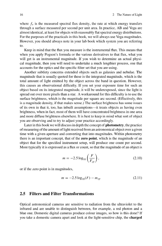
More typically it is expressed as a flux or count, so that the magnitude of an object is
m = −2.5 log 10
F
F zp
,
(2.10)
or if the zero point is in magnitudes,
m = −2.5 log 10 (F) − m zp
(2.11)
2.5 Filters and Filter Transformations
Optical astronomical cameras are sensitive to radiation from the ultraviolet to the
infrared and are unable to distinguish between, for example, a red photon and a
blue one. Domestic digital cameras produce colour images, so how is this done? If
you take a domestic camera apart and look at the light-sensitive chip, the charged
2 The Nature of Light
where f v is the measured spectral flux density, the rate at which energy transfers
through a surface measured per second per unit area. In practice, AB and Vega are
almost identical, at least for objects with reasonably flat spectral energy distributions.
For the purposes of the practicals in this book, we will always use Vega magnitudes.
However, you should always note in your lab book which system you are referring
to.
Keep in mind that the flux you measure is the instrumental flux. This means that
when you apply Pogson’s formula or the various derivatives to that flux, what you
will get is an instrumental magnitude. If you wish to determine an actual physical magnitude, then you will need to undertake a much lengthier process, one that
accounts for the optics and the specific filter set that you are using.
Another subtlety concerns extended objects such as galaxies and nebulae. The
magnitude that is usually quoted for these is the integrated magnitude, which is the
total amount of light emitted by the object across the band in question. However,
this causes an observational difficulty. If you set your exposure time for such an
object based on its integrated magnitude, it will be underexposed, since the light is
spread out over more pixels than a star. A workaround for this difficulty is to use the
surface brightness, which is the magnitude per square arc second. (Effectively, this
is a magnitude density, if that makes sense.) The surface brightness has some issues
of its own in that it, too, has inbuilt assumptions—it treats objects as having even
brightness, when in fact, most of them will have concentrated brightness in one area
and more diffuse brightness elsewhere. It is best to keep in mind what sort of object
you are observing and to try to adjust your practice accordingly.
Later in this book we will discuss in depth the concept of photometry, the practice
of measuring of the amount of light received from an astronomical object over a given
time with a given aperture and converting that into magnitudes. Within photometry
there is an important concept, that of the zero point, which is the magnitude of an
object that for the specified instrument setup, will produce one count per second.
More typically it is expressed as a flux or count, so that the magnitude of an object is
m = −2.5 log 10
F
F zp
,
(2.10)
or if the zero point is in magnitudes,
m = −2.5 log 10 (F) − m zp
(2.11)
2.5 Filters and Filter Transformations
Optical astronomical cameras are sensitive to radiation from the ultraviolet to the
infrared and are unable to distinguish between, for example, a red photon and a
blue one. Domestic digital cameras produce colour images, so how is this done? If
you take a domestic camera apart and look at the light-sensitive chip, the charged