

11.3 Handling Errors
163
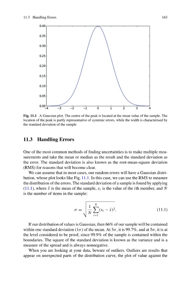
Fig. 11.1 A Gaussian plot. The centre of the peak is located at the mean value of the sample. The
location of the peak is partly representative of systemic errors, while the width is characterised by
the standard deviation of the sample
11.3 Handling Errors
One of the most common methods of finding uncertainties is to make multiple measurements and take the mean or median as the result and the standard deviation as
the error. The standard deviation is also known as the root-mean-square deviation
(RMS) for reasons that will become clear.
We can assume that in most cases, our random errors will have a Gaussian distribution, whose plot looks like Fig. 11.1. In this case, we can use the RMS to measure
the distribution of the errors. The standard deviation of a sample is found by applying
(11.1), where ¯
x is the mean of the sample, x i is the value of the ith member, and N
is the number of items in the sample:
σ =
1
N
N
i=1
(x i − ¯
x) 2 .
(11.1)
If our distribution of values is Gaussian, then 66% of our sample will be contained
within one standard deviation (1σ ) of the mean. At 3σ , it is 99.7%, and at 5σ , it is at
the level considered to be proof, since 99.9% of the sample is contained within the
boundaries. The square of the standard deviation is known as the variance and is a
measure of the spread and is always nonnegative.
When you are looking at your data, beware of outliers. Outliers are results that
appear on unexpected parts of the distribution curve, the plot of value against the
163
Fig. 11.1 A Gaussian plot. The centre of the peak is located at the mean value of the sample. The
location of the peak is partly representative of systemic errors, while the width is characterised by
the standard deviation of the sample
11.3 Handling Errors
One of the most common methods of finding uncertainties is to make multiple measurements and take the mean or median as the result and the standard deviation as
the error. The standard deviation is also known as the root-mean-square deviation
(RMS) for reasons that will become clear.
We can assume that in most cases, our random errors will have a Gaussian distribution, whose plot looks like Fig. 11.1. In this case, we can use the RMS to measure
the distribution of the errors. The standard deviation of a sample is found by applying
(11.1), where ¯
x is the mean of the sample, x i is the value of the ith member, and N
is the number of items in the sample:
σ =
1
N
N
i=1
(x i − ¯
x) 2 .
(11.1)
If our distribution of values is Gaussian, then 66% of our sample will be contained
within one standard deviation (1σ ) of the mean. At 3σ , it is 99.7%, and at 5σ , it is at
the level considered to be proof, since 99.9% of the sample is contained within the
boundaries. The square of the standard deviation is known as the variance and is a
measure of the spread and is always nonnegative.
When you are looking at your data, beware of outliers. Outliers are results that
appear on unexpected parts of the distribution curve, the plot of value against the