

3.17 Numerical Examples
83
l 3 = 0, m 3 = 0, n 3 = 1
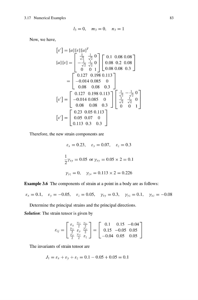
Now, we have,
ε
= [a] [ε] [a]
T
[a] [ε] =
⎡
⎢
⎣
1
√
2
1
√
2
0
−
1
√
2
1
√
2
0
0 0 1
⎤
⎥
⎦
⎡
⎣
0.1 0.08 0.08
0.08 0.2 0.08
0.08 0.08 0.3
⎤
⎦
=
⎡
⎣
0.127 0.198 0.113
−0.014 0.085 0
0.08 0.08 0.3
⎤
⎦
ε
=
⎡
⎣
0.127 0.198 0.113
−0.014 0.085 0
0.08 0.08 0.3
⎤
⎦
⎡
⎢
⎣
1
√
2
−
1
√
2
0
1
√
2
1
√
2
0
0 0 1
⎤
⎥
⎦
ε
=
⎡
⎣
0.23 0.05 0.113
0.05 0.07 0
0.113 0.3 0.3
⎤
⎦
Therefore, the new strain components are
ε x = 0.23, ε y = 0.07, ε z = 0.3
1
2
γ xy = 0.05 or γ xy = 0.05 × 2 = 0.1
γ yz = 0, γ zx = 0.113 × 2 = 0.226
Example 3.6 The components of strain at a point in a body are as follows:
ε x = 0.1, ε y = −0.05, ε z = 0.05, γ xy = 0.3, γ yz = 0.1, γ xz = −0.08
Determine the principal strains and the principal directions.
Solution: The strain tensor is given by
ε i j =
⎡
⎣
ε x
γ xy
2
γ xz
2
γ xy
2
ε y
γ yz
2
γ xz
2
γ yz
2
ε z
⎤
⎦ =
⎡
⎣
0.1 0.15 −0.04
0.15 −0.05 0.05
−0.04 0.05 0.05
⎤
⎦
The invariants of strain tensor are
J 1 = ε x + ε y + ε z = 0.1 − 0.05 + 0.05 = 0.1
83
l 3 = 0, m 3 = 0, n 3 = 1
Now, we have,
ε
= [a] [ε] [a]
T
[a] [ε] =
⎡
⎢
⎣
1
√
2
1
√
2
0
−
1
√
2
1
√
2
0
0 0 1
⎤
⎥
⎦
⎡
⎣
0.1 0.08 0.08
0.08 0.2 0.08
0.08 0.08 0.3
⎤
⎦
=
⎡
⎣
0.127 0.198 0.113
−0.014 0.085 0
0.08 0.08 0.3
⎤
⎦
ε
=
⎡
⎣
0.127 0.198 0.113
−0.014 0.085 0
0.08 0.08 0.3
⎤
⎦
⎡
⎢
⎣
1
√
2
−
1
√
2
0
1
√
2
1
√
2
0
0 0 1
⎤
⎥
⎦
ε
=
⎡
⎣
0.23 0.05 0.113
0.05 0.07 0
0.113 0.3 0.3
⎤
⎦
Therefore, the new strain components are
ε x = 0.23, ε y = 0.07, ε z = 0.3
1
2
γ xy = 0.05 or γ xy = 0.05 × 2 = 0.1
γ yz = 0, γ zx = 0.113 × 2 = 0.226
Example 3.6 The components of strain at a point in a body are as follows:
ε x = 0.1, ε y = −0.05, ε z = 0.05, γ xy = 0.3, γ yz = 0.1, γ xz = −0.08
Determine the principal strains and the principal directions.
Solution: The strain tensor is given by
ε i j =
⎡
⎣
ε x
γ xy
2
γ xz
2
γ xy
2
ε y
γ yz
2
γ xz
2
γ yz
2
ε z
⎤
⎦ =
⎡
⎣
0.1 0.15 −0.04
0.15 −0.05 0.05
−0.04 0.05 0.05
⎤
⎦
The invariants of strain tensor are
J 1 = ε x + ε y + ε z = 0.1 − 0.05 + 0.05 = 0.1