

44
2 Analysis of Stress
x
y
z
x
0.866
0.5
0
y
−0.5
0.866
0
z
0
0
1
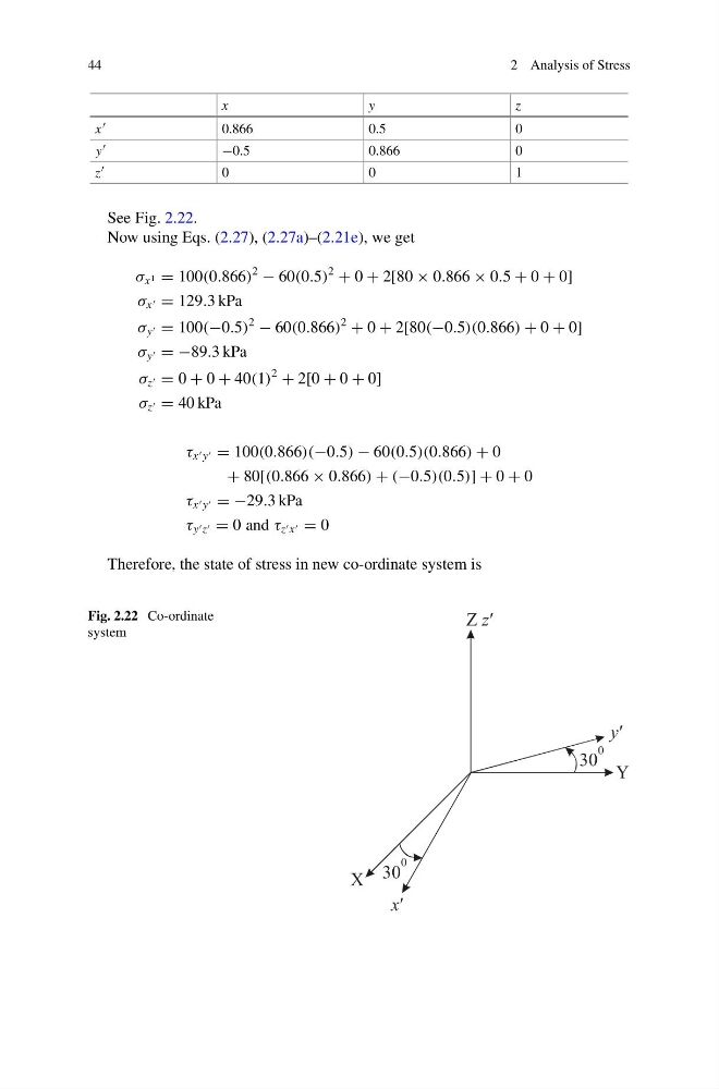
See Fig. 2.22.
Now using Eqs. (2.27), (2.27a)–(2.21e), we get
σ x 1 = 100(0.866)
2
− 60(0.5)
2
+ 0 + 2[80 × 0.866 × 0.5 + 0 + 0]
σ x = 129.3 kPa
σ y = 100(−0.5)
2
− 60(0.866)
2
+ 0 + 2[80(−0.5)(0.866) + 0 + 0]
σ y = −89.3 kPa
σ z = 0 + 0 + 40(1)
2
+ 2[0 + 0 + 0]
σ z = 40 kPa
τ x y = 100(0.866)(−0.5) − 60(0.5)(0.866) + 0
+ 80[(0.866 × 0.866) + (−0.5)(0.5)] + 0 + 0
τ x y = −29.3 kPa
τ y z = 0 and τ z x = 0
Therefore, the state of stress in new co-ordinate system is
Fig. 2.22 Co-ordinate
system
2 Analysis of Stress
x
y
z
x
0.866
0.5
0
y
−0.5
0.866
0
z
0
0
1
See Fig. 2.22.
Now using Eqs. (2.27), (2.27a)–(2.21e), we get
σ x 1 = 100(0.866)
2
− 60(0.5)
2
+ 0 + 2[80 × 0.866 × 0.5 + 0 + 0]
σ x = 129.3 kPa
σ y = 100(−0.5)
2
− 60(0.866)
2
+ 0 + 2[80(−0.5)(0.866) + 0 + 0]
σ y = −89.3 kPa
σ z = 0 + 0 + 40(1)
2
+ 2[0 + 0 + 0]
σ z = 40 kPa
τ x y = 100(0.866)(−0.5) − 60(0.5)(0.866) + 0
+ 80[(0.866 × 0.866) + (−0.5)(0.5)] + 0 + 0
τ x y = −29.3 kPa
τ y z = 0 and τ z x = 0
Therefore, the state of stress in new co-ordinate system is
Fig. 2.22 Co-ordinate
system