

8.2 Kelvin’s Problem
263
τ r θ = τ θr = τ θ z = τ zθ = 0
Here, R =
√
z 2 + r 2
From the above expressions, it is clear that both displacements and stresses reduce
to zero for larger values of R. However, on the plane z =0, all the stress components
except for τ rz vanish, at all points except the origin.
Vertical Tractions Equilibrating the Applied Point Load
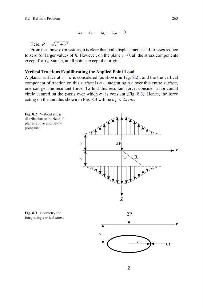
A planar surface at z = h is considered (as shown in Fig. 8.2), and the the vertical
component of traction on this surface is σ z . integrating σ z ; over this entire surface,
one can get the resultant force. To find this resultant force, consider a horizontal
circle centred on the z-axis over which σ z is constant (Fig. 8.3). Hence, the force
acting on the annulus shown in Fig. 8.3 will be σ z × 2π rdr.
Fig. 8.2 Vertical stress
distribution on horizontal
planes above and below
point load
Fig. 8.3 Geometry for
integrating vertical stress
r
r
dr
Z
2P
h
263
τ r θ = τ θr = τ θ z = τ zθ = 0
Here, R =
√
z 2 + r 2
From the above expressions, it is clear that both displacements and stresses reduce
to zero for larger values of R. However, on the plane z =0, all the stress components
except for τ rz vanish, at all points except the origin.
Vertical Tractions Equilibrating the Applied Point Load
A planar surface at z = h is considered (as shown in Fig. 8.2), and the the vertical
component of traction on this surface is σ z . integrating σ z ; over this entire surface,
one can get the resultant force. To find this resultant force, consider a horizontal
circle centred on the z-axis over which σ z is constant (Fig. 8.3). Hence, the force
acting on the annulus shown in Fig. 8.3 will be σ z × 2π rdr.
Fig. 8.2 Vertical stress
distribution on horizontal
planes above and below
point load
Fig. 8.3 Geometry for
integrating vertical stress
r
r
dr
Z
2P
h