

5.9 Numerical Examples
159
Hence, the stress components are
σ x =
∂
2
φ
∂ y 2 = p − 1.5
F
h 3 x y
σ y =
∂
2
φ
∂ x 2 = 0
τ xy = −
∂
2
φ
∂ x∂ y
=
3
4
F y
2
h 3 −
3F
4h
(a) Variation of σ x (Fig 5.14)
σ x = p −
1.5
F
h 3
x y
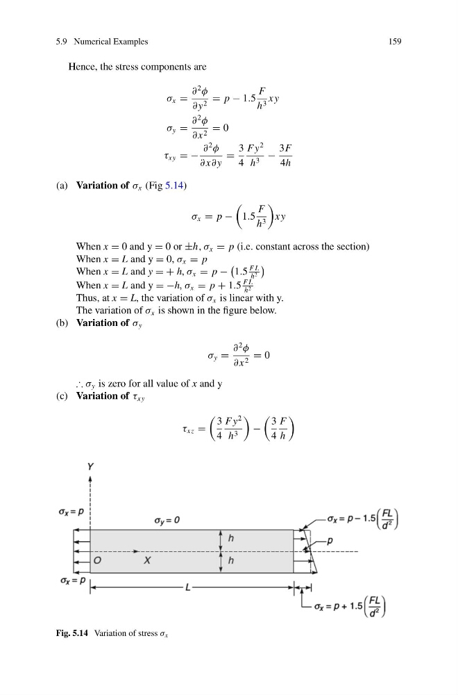
When x = 0 and y = 0 or ±h, σ x = p (i.e. constant across the section)
When x = L and y = 0, σ x = p
When x = L and y = + h, σ x = p −
1.5
F L
h 2
When x = L and y = −h, σ x = p + 1.5
F L
h 2
Thus, at x = L, the variation of σ x is linear with y.
The variation of σ x is shown in the figure below.
(b) Variation of σ y
σ y =
∂
2
φ
∂ x 2 = 0
∴ σ y is zero for all value of x and y
(c) Variation of τ xy
τ xz =
3
4
F y
2
h 3
−
3
4
F
h
Fig. 5.14 Variation of stress σ x
159
Hence, the stress components are
σ x =
∂
2
φ
∂ y 2 = p − 1.5
F
h 3 x y
σ y =
∂
2
φ
∂ x 2 = 0
τ xy = −
∂
2
φ
∂ x∂ y
=
3
4
F y
2
h 3 −
3F
4h
(a) Variation of σ x (Fig 5.14)
σ x = p −
1.5
F
h 3
x y
When x = 0 and y = 0 or ±h, σ x = p (i.e. constant across the section)
When x = L and y = 0, σ x = p
When x = L and y = + h, σ x = p −
1.5
F L
h 2
When x = L and y = −h, σ x = p + 1.5
F L
h 2
Thus, at x = L, the variation of σ x is linear with y.
The variation of σ x is shown in the figure below.
(b) Variation of σ y
σ y =
∂
2
φ
∂ x 2 = 0
∴ σ y is zero for all value of x and y
(c) Variation of τ xy
τ xz =
3
4
F y
2
h 3
−
3
4
F
h
Fig. 5.14 Variation of stress σ x