

5.9 Numerical Examples
157
and
∂
2 φ
∂ x 2 = 0
also
∂
2 φ
∂ x∂ y
= −
6Fz
h 2
+
6F
h 3
y
2 .
Hence,
σ x = −
6F x
h 2
+
12F
h 3
x y
(i)
σ y = 0
( i i )
τ xy = −
∂
2
φ
∂ x∂ y
= −
6F y
h 2
+
6F
h 3
y
2
(iii)
Variation of Stresses at Certain Boundary Points
(a) Variation of σ x
From (i), it is clear that σ x varies linearly with x, and at a given section it varies
linearly with z.
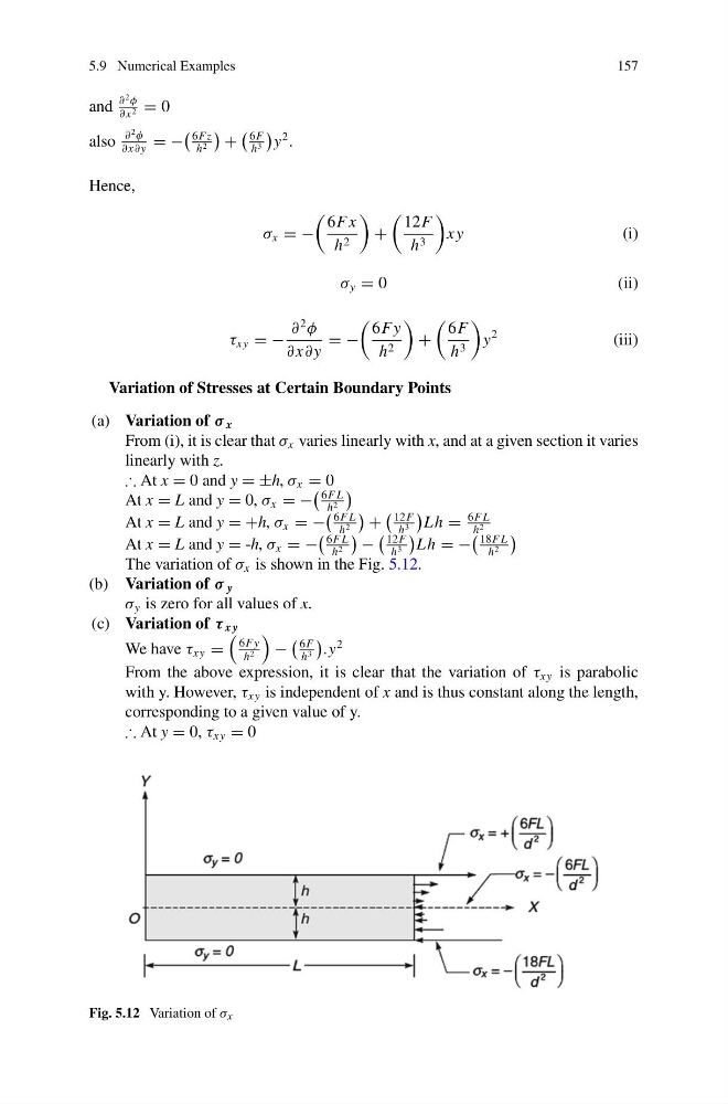
∴ At x = 0 and y = ±h, σ x = 0
At x = L and y = 0, σ x = −
6F L
h 2
At x = L and y = +h, σ x = −
6F L
h 2
+
12F
h 3
Lh =
6F L
h 2
At x = L and y = -h, σ x = −
6F L
h 2
−
12F
h 3
Lh = −
18F L
h 2
The variation of σ x is shown in the Fig. 5.12.
(b) Variation of σ y
σ y is zero for all values of x.
(c) Variation of τ x y
We have τ xy =
6Fy
h 2
−
6F
h 3
.y
2
From the above expression, it is clear that the variation of τ xy is parabolic
with y. However, τ xy is independent of x and is thus constant along the length,
corresponding to a given value of y.
∴ At y = 0, τ xy = 0
Fig. 5.12 Variation of σ x
157
and
∂
2 φ
∂ x 2 = 0
also
∂
2 φ
∂ x∂ y
= −
6Fz
h 2
+
6F
h 3
y
2 .
Hence,
σ x = −
6F x
h 2
+
12F
h 3
x y
(i)
σ y = 0
( i i )
τ xy = −
∂
2
φ
∂ x∂ y
= −
6F y
h 2
+
6F
h 3
y
2
(iii)
Variation of Stresses at Certain Boundary Points
(a) Variation of σ x
From (i), it is clear that σ x varies linearly with x, and at a given section it varies
linearly with z.
∴ At x = 0 and y = ±h, σ x = 0
At x = L and y = 0, σ x = −
6F L
h 2
At x = L and y = +h, σ x = −
6F L
h 2
+
12F
h 3
Lh =
6F L
h 2
At x = L and y = -h, σ x = −
6F L
h 2
−
12F
h 3
Lh = −
18F L
h 2
The variation of σ x is shown in the Fig. 5.12.
(b) Variation of σ y
σ y is zero for all values of x.
(c) Variation of τ x y
We have τ xy =
6Fy
h 2
−
6F
h 3
.y
2
From the above expression, it is clear that the variation of τ xy is parabolic
with y. However, τ xy is independent of x and is thus constant along the length,
corresponding to a given value of y.
∴ At y = 0, τ xy = 0
Fig. 5.12 Variation of σ x