

90
5 General-Relativistic Matrix Kinetic Theory
m s = m s
⇒
f ss | s =s ≡ 0 ,
(5.2.15)
just as the selection rules we already have for Grassmann parity (5.2.2) and charge
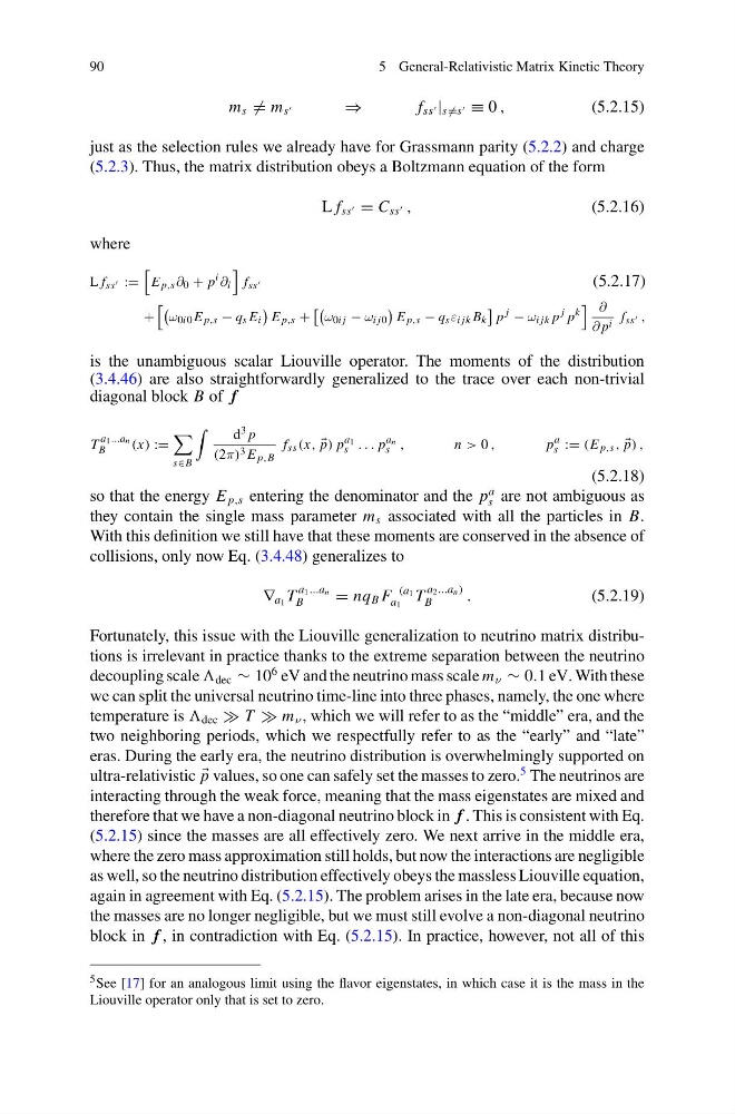
(5.2.3). Thus, the matrix distribution obeys a Boltzmann equation of the form
L f ss = C ss ,
(5.2.16)
where
L f ss :=
E p,s ∂ 0 + p
i ∂ i
f ss
(5.2.17)
+
ω 0i0 E p,s − q s E i
E p,s +
ω 0i j − ω i j0
E p,s − q s ε i jk B k
p
j − ω i jk p
j p
k
∂
∂ p i f ss ,
is the unambiguous scalar Liouville operator. The moments of the distribution
(3.4.46) are also straightforwardly generalized to the trace over each non-trivial
diagonal block B of f
T
a1...an
B
(x) :=
s∈B
d 3 p
(2π) 3 E p,B
f ss (x,
p) p
a1
s . . . p
an
s ,
n > 0 ,
p
a
s := (E p,s ,
p) ,
(5.2.18)
so that the energy E p,s entering the denominator and the p
a
s are not ambiguous as
they contain the single mass parameter m s associated with all the particles in B.
With this definition we still have that these moments are conserved in the absence of
collisions, only now Eq. (3.4.48) generalizes to
∇ a 1 T
a 1 ...a n
B
= nq B F
(a 1
a 1
T
a 2 ...a n )
B
.
(5.2.19)
Fortunately, this issue with the Liouville generalization to neutrino matrix distributions is irrelevant in practice thanks to the extreme separation between the neutrino
decoupling scale dec ∼ 10
6 eV and the neutrino mass scale m ν ∼ 0.1 eV. With these
we can split the universal neutrino time-line into three phases, namely, the one where
temperature is dec T m ν , which we will refer to as the “middle” era, and the
two neighboring periods, which we respectfully refer to as the “early” and “late”
eras. During the early era, the neutrino distribution is overwhelmingly supported on
ultra-relativistic
p values, so one can safely set the masses to zero.
5 The neutrinos are
interacting through the weak force, meaning that the mass eigenstates are mixed and
therefore that we have a non-diagonal neutrino block in f . This is consistent with Eq.
(5.2.15) since the masses are all effectively zero. We next arrive in the middle era,
where the zero mass approximation still holds, but now the interactions are negligible
as well, so the neutrino distribution effectively obeys the massless Liouville equation,
again in agreement with Eq. (5.2.15). The problem arises in the late era, because now
the masses are no longer negligible, but we must still evolve a non-diagonal neutrino
block in f , in contradiction with Eq. (5.2.15). In practice, however, not all of this
5 See [17] for an analogous limit using the flavor eigenstates, in which case it is the mass in the
Liouville operator only that is set to zero.
5 General-Relativistic Matrix Kinetic Theory
m s = m s
⇒
f ss | s =s ≡ 0 ,
(5.2.15)
just as the selection rules we already have for Grassmann parity (5.2.2) and charge
(5.2.3). Thus, the matrix distribution obeys a Boltzmann equation of the form
L f ss = C ss ,
(5.2.16)
where
L f ss :=
E p,s ∂ 0 + p
i ∂ i
f ss
(5.2.17)
+
ω 0i0 E p,s − q s E i
E p,s +
ω 0i j − ω i j0
E p,s − q s ε i jk B k
p
j − ω i jk p
j p
k
∂
∂ p i f ss ,
is the unambiguous scalar Liouville operator. The moments of the distribution
(3.4.46) are also straightforwardly generalized to the trace over each non-trivial
diagonal block B of f
T
a1...an
B
(x) :=
s∈B
d 3 p
(2π) 3 E p,B
f ss (x,
p) p
a1
s . . . p
an
s ,
n > 0 ,
p
a
s := (E p,s ,
p) ,
(5.2.18)
so that the energy E p,s entering the denominator and the p
a
s are not ambiguous as
they contain the single mass parameter m s associated with all the particles in B.
With this definition we still have that these moments are conserved in the absence of
collisions, only now Eq. (3.4.48) generalizes to
∇ a 1 T
a 1 ...a n
B
= nq B F
(a 1
a 1
T
a 2 ...a n )
B
.
(5.2.19)
Fortunately, this issue with the Liouville generalization to neutrino matrix distributions is irrelevant in practice thanks to the extreme separation between the neutrino
decoupling scale dec ∼ 10
6 eV and the neutrino mass scale m ν ∼ 0.1 eV. With these
we can split the universal neutrino time-line into three phases, namely, the one where
temperature is dec T m ν , which we will refer to as the “middle” era, and the
two neighboring periods, which we respectfully refer to as the “early” and “late”
eras. During the early era, the neutrino distribution is overwhelmingly supported on
ultra-relativistic
p values, so one can safely set the masses to zero.
5 The neutrinos are
interacting through the weak force, meaning that the mass eigenstates are mixed and
therefore that we have a non-diagonal neutrino block in f . This is consistent with Eq.
(5.2.15) since the masses are all effectively zero. We next arrive in the middle era,
where the zero mass approximation still holds, but now the interactions are negligible
as well, so the neutrino distribution effectively obeys the massless Liouville equation,
again in agreement with Eq. (5.2.15). The problem arises in the late era, because now
the masses are no longer negligible, but we must still evolve a non-diagonal neutrino
block in f , in contradiction with Eq. (5.2.15). In practice, however, not all of this
5 See [17] for an analogous limit using the flavor eigenstates, in which case it is the mass in the
Liouville operator only that is set to zero.