

58
4 Observer Space-Time Formalism
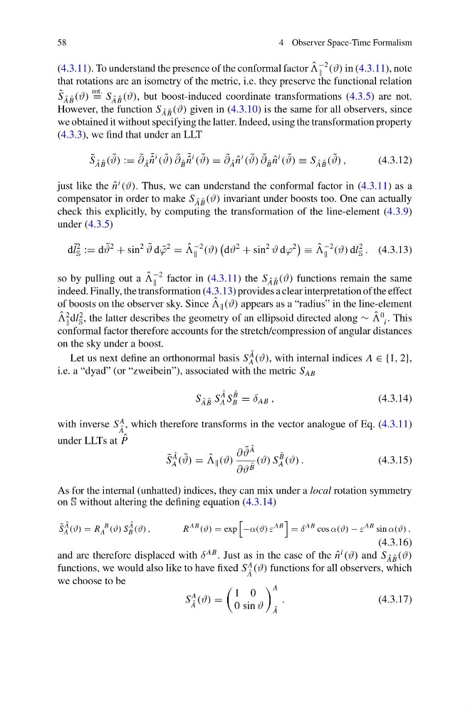
(4.3.11). To understand the presence of the conformal factor ˆ
−2
(ϑ) in (4.3.11), note
that rotations are an isometry of the metric, i.e. they preserve the functional relation
˜
S ˆ
A ˆ
B (ϑ)
rot.
= S ˆ
A ˆ
B (ϑ), but boost-induced coordinate transformations (4.3.5) are not.
However, the function S ˆ
A ˆ
B (ϑ) given in (4.3.10) is the same for all observers, since
we obtained it without specifying the latter. Indeed, using the transformation property
(4.3.3), we find that under an LLT
˜
S ˆ
A ˆ
B ( ˜
ϑ) := ˜
∂ ˆ
A
˜ ˆ
n
i
( ˜
ϑ) ˜
∂ ˆ
B
˜ ˆ
n
i
( ˜
ϑ) = ˜
∂ ˆ
A ˆ
n
i
( ˜
ϑ) ˜
∂ ˆ
B ˆ
n
i
( ˜
ϑ) ≡ S ˆ
A ˆ
B ( ˜
ϑ) ,
(4.3.12)
just like the ˆ
n
i
(ϑ). Thus, we can understand the conformal factor in (4.3.11) as a
compensator in order to make S ˆ
A ˆ
B (ϑ) invariant under boosts too. One can actually
check this explicitly, by computing the transformation of the line-element (4.3.9)
under (4.3.5)
d ˜
l
2
S := d ˜
ϑ
2
+ sin
2 ˜
ϑ d ˜
ϕ
2
= ˆ
−2
(ϑ)
dϑ
2
+ sin
2
ϑ dϕ
2
≡ ˆ
−2
(ϑ) dl
2
S . (4.3.13)
so by pulling out a ˆ
−2
factor in (4.3.11) the S ˆ
A ˆ
B (ϑ) functions remain the same
indeed. Finally, the transformation (4.3.13) provides a clear interpretation of the effect
of boosts on the observer sky. Since ˆ
(ϑ) appears as a “radius” in the line-element
ˆ
2
dl
2
S , the latter describes the geometry of an ellipsoid directed along ∼ ˆ
0
i . This
conformal factor therefore accounts for the stretch/compression of angular distances
on the sky under a boost.
Let us next define an orthonormal basis S
ˆ
A
A (ϑ), with internal indices A ∈ {1, 2},
i.e. a “dyad” (or “zweibein”), associated with the metric S AB
S ˆ
A ˆ
B S
ˆ
A
A S
ˆ
B
B = δ AB ,
(4.3.14)
with inverse S
A
ˆ
A
, which therefore transforms in the vector analogue of Eq. (4.3.11)
under LLTs at ˆ
P
˜
S
ˆ
A
A ( ˜
ϑ) = ˆ
(ϑ)
∂ ˜
ϑ
ˆ
A
∂ϑ
ˆ
B
(ϑ) S
ˆ
B
A (ϑ) .
(4.3.15)
As for the internal (unhatted) indices, they can mix under a local rotation symmetry
on S without altering the defining equation (4.3.14)
˜
S
ˆ
A
A (ϑ) = R
B
A (ϑ) S
ˆ
A
B (ϑ) ,
R
AB (ϑ) = exp
−α(ϑ) ε
AB
= δ
AB cos α(ϑ) − ε
AB sin α(ϑ) ,
(4.3.16)
and are therefore displaced with δ
AB . Just as in the case of the ˆ
n
i
(ϑ) and S ˆ
A ˆ
B (ϑ)
functions, we would also like to have fixed S
A
ˆ
A
(ϑ) functions for all observers, which
we choose to be
S
A
ˆ
A
(ϑ) =
1 0
0 sin ϑ
A
ˆ
A
.
(4.3.17)
4 Observer Space-Time Formalism
(4.3.11). To understand the presence of the conformal factor ˆ
−2
(ϑ) in (4.3.11), note
that rotations are an isometry of the metric, i.e. they preserve the functional relation
˜
S ˆ
A ˆ
B (ϑ)
rot.
= S ˆ
A ˆ
B (ϑ), but boost-induced coordinate transformations (4.3.5) are not.
However, the function S ˆ
A ˆ
B (ϑ) given in (4.3.10) is the same for all observers, since
we obtained it without specifying the latter. Indeed, using the transformation property
(4.3.3), we find that under an LLT
˜
S ˆ
A ˆ
B ( ˜
ϑ) := ˜
∂ ˆ
A
˜ ˆ
n
i
( ˜
ϑ) ˜
∂ ˆ
B
˜ ˆ
n
i
( ˜
ϑ) = ˜
∂ ˆ
A ˆ
n
i
( ˜
ϑ) ˜
∂ ˆ
B ˆ
n
i
( ˜
ϑ) ≡ S ˆ
A ˆ
B ( ˜
ϑ) ,
(4.3.12)
just like the ˆ
n
i
(ϑ). Thus, we can understand the conformal factor in (4.3.11) as a
compensator in order to make S ˆ
A ˆ
B (ϑ) invariant under boosts too. One can actually
check this explicitly, by computing the transformation of the line-element (4.3.9)
under (4.3.5)
d ˜
l
2
S := d ˜
ϑ
2
+ sin
2 ˜
ϑ d ˜
ϕ
2
= ˆ
−2
(ϑ)
dϑ
2
+ sin
2
ϑ dϕ
2
≡ ˆ
−2
(ϑ) dl
2
S . (4.3.13)
so by pulling out a ˆ
−2
factor in (4.3.11) the S ˆ
A ˆ
B (ϑ) functions remain the same
indeed. Finally, the transformation (4.3.13) provides a clear interpretation of the effect
of boosts on the observer sky. Since ˆ
(ϑ) appears as a “radius” in the line-element
ˆ
2
dl
2
S , the latter describes the geometry of an ellipsoid directed along ∼ ˆ
0
i . This
conformal factor therefore accounts for the stretch/compression of angular distances
on the sky under a boost.
Let us next define an orthonormal basis S
ˆ
A
A (ϑ), with internal indices A ∈ {1, 2},
i.e. a “dyad” (or “zweibein”), associated with the metric S AB
S ˆ
A ˆ
B S
ˆ
A
A S
ˆ
B
B = δ AB ,
(4.3.14)
with inverse S
A
ˆ
A
, which therefore transforms in the vector analogue of Eq. (4.3.11)
under LLTs at ˆ
P
˜
S
ˆ
A
A ( ˜
ϑ) = ˆ
(ϑ)
∂ ˜
ϑ
ˆ
A
∂ϑ
ˆ
B
(ϑ) S
ˆ
B
A (ϑ) .
(4.3.15)
As for the internal (unhatted) indices, they can mix under a local rotation symmetry
on S without altering the defining equation (4.3.14)
˜
S
ˆ
A
A (ϑ) = R
B
A (ϑ) S
ˆ
A
B (ϑ) ,
R
AB (ϑ) = exp
−α(ϑ) ε
AB
= δ
AB cos α(ϑ) − ε
AB sin α(ϑ) ,
(4.3.16)
and are therefore displaced with δ
AB . Just as in the case of the ˆ
n
i
(ϑ) and S ˆ
A ˆ
B (ϑ)
functions, we would also like to have fixed S
A
ˆ
A
(ϑ) functions for all observers, which
we choose to be
S
A
ˆ
A
(ϑ) =
1 0
0 sin ϑ
A
ˆ
A
.
(4.3.17)