

56
4 Observer Space-Time Formalism
4.3 Observer Sky
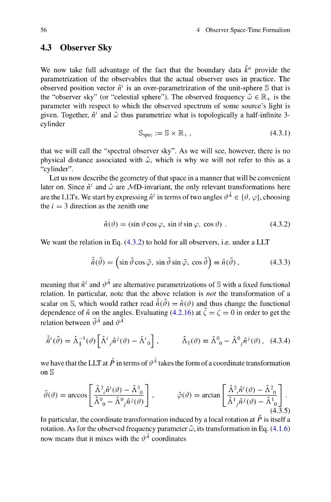
We now take full advantage of the fact that the boundary data ˆ
k
a provide the
parametrization of the observables that the actual observer uses in practice. The
observed position vector ˆ
n
i is an over-parametrization of the unit-sphere S that is
the “observer sky” (or “celestial sphere”). The observed frequency ˆ
ω ∈ R + is the
parameter with respect to which the observed spectrum of some source’s light is
given. Together, ˆ
n
i and ˆ
ω thus parametrize what is topologically a half-infinite 3cylinder
S spec := S × R + ,
(4.3.1)
that we will call the “spectral observer sky”. As we will see, however, there is no
physical distance associated with ˆ
ω, which is why we will not refer to this as a
“cylinder”.
Let us now describe the geometry of that space in a manner that will be convenient
later on. Since ˆ
n
i and ˆ
ω are MD-invariant, the only relevant transformations here
are the LLTs. We start by expressing ˆ
n
i in terms of two angles ϑ
ˆ
A
∈ {ϑ, ϕ}, choosing
the i = 3 direction as the zenith one
ˆ
n(ϑ) = (sin ϑ cos ϕ, sin ϑ sin ϕ, cos ϑ) .
(4.3.2)
We want the relation in Eq. (4.3.2) to hold for all observers, i.e. under a LLT
˜ ˆ
n( ˜
ϑ) =
sin ˜
ϑ cos ˜
ϕ, sin ˜
ϑ sin ˜
ϕ, cos ˜
ϑ
≡ ˆ
n( ˜
ϑ) ,
(4.3.3)
meaning that ˆ
n
i and ϑ
ˆ
A are alternative parametrizations of S with a fixed functional
relation. In particular, note that the above relation is not the transformation of a
scalar on S, which would rather read ˜ ˆ
n( ˜
ϑ) = ˆ
n(ϑ) and thus change the functional
dependence of ˆ
n on the angles. Evaluating (4.2.16) at ˜
ζ = ζ = 0 in order to get the
relation between ˜
ϑ
ˆ
A and ϑ
ˆ
A
˜ ˆ
n
i
( ˜
ϑ) = ˆ
−1
(ϑ)
ˆ
i
j ˆ
n
j
(ϑ) − ˆ
i
0
,
ˆ
(ϑ) ≡ ˆ
0
0 − ˆ
0
j ˆ
n
j
(ϑ) , (4.3.4)
we have that the LLT at ˆ
P in terms of ϑ
ˆ
A takes the form of a coordinate transformation
on S
˜
ϑ(ϑ) = arccos
ˆ
3
i ˆ
n
i
(ϑ) − ˆ
3
0
ˆ
0
0 − ˆ
0
j ˆ
n j (ϑ)
,
˜
ϕ(ϑ) = arctan
ˆ
2
i ˆ
n
i
(ϑ) − ˆ
2
0
ˆ
1
j ˆ
n j (ϑ) − ˆ
1
0
.
(4.3.5)
In particular, the coordinate transformation induced by a local rotation at ˆ
P is itself a
rotation. As for the observed frequency parameter ˆ
ω, its transformation in Eq. (4.1.6)
now means that it mixes with the ϑ
ˆ
A coordinates
4 Observer Space-Time Formalism
4.3 Observer Sky
We now take full advantage of the fact that the boundary data ˆ
k
a provide the
parametrization of the observables that the actual observer uses in practice. The
observed position vector ˆ
n
i is an over-parametrization of the unit-sphere S that is
the “observer sky” (or “celestial sphere”). The observed frequency ˆ
ω ∈ R + is the
parameter with respect to which the observed spectrum of some source’s light is
given. Together, ˆ
n
i and ˆ
ω thus parametrize what is topologically a half-infinite 3cylinder
S spec := S × R + ,
(4.3.1)
that we will call the “spectral observer sky”. As we will see, however, there is no
physical distance associated with ˆ
ω, which is why we will not refer to this as a
“cylinder”.
Let us now describe the geometry of that space in a manner that will be convenient
later on. Since ˆ
n
i and ˆ
ω are MD-invariant, the only relevant transformations here
are the LLTs. We start by expressing ˆ
n
i in terms of two angles ϑ
ˆ
A
∈ {ϑ, ϕ}, choosing
the i = 3 direction as the zenith one
ˆ
n(ϑ) = (sin ϑ cos ϕ, sin ϑ sin ϕ, cos ϑ) .
(4.3.2)
We want the relation in Eq. (4.3.2) to hold for all observers, i.e. under a LLT
˜ ˆ
n( ˜
ϑ) =
sin ˜
ϑ cos ˜
ϕ, sin ˜
ϑ sin ˜
ϕ, cos ˜
ϑ
≡ ˆ
n( ˜
ϑ) ,
(4.3.3)
meaning that ˆ
n
i and ϑ
ˆ
A are alternative parametrizations of S with a fixed functional
relation. In particular, note that the above relation is not the transformation of a
scalar on S, which would rather read ˜ ˆ
n( ˜
ϑ) = ˆ
n(ϑ) and thus change the functional
dependence of ˆ
n on the angles. Evaluating (4.2.16) at ˜
ζ = ζ = 0 in order to get the
relation between ˜
ϑ
ˆ
A and ϑ
ˆ
A
˜ ˆ
n
i
( ˜
ϑ) = ˆ
−1
(ϑ)
ˆ
i
j ˆ
n
j
(ϑ) − ˆ
i
0
,
ˆ
(ϑ) ≡ ˆ
0
0 − ˆ
0
j ˆ
n
j
(ϑ) , (4.3.4)
we have that the LLT at ˆ
P in terms of ϑ
ˆ
A takes the form of a coordinate transformation
on S
˜
ϑ(ϑ) = arccos
ˆ
3
i ˆ
n
i
(ϑ) − ˆ
3
0
ˆ
0
0 − ˆ
0
j ˆ
n j (ϑ)
,
˜
ϕ(ϑ) = arctan
ˆ
2
i ˆ
n
i
(ϑ) − ˆ
2
0
ˆ
1
j ˆ
n j (ϑ) − ˆ
1
0
.
(4.3.5)
In particular, the coordinate transformation induced by a local rotation at ˆ
P is itself a
rotation. As for the observed frequency parameter ˆ
ω, its transformation in Eq. (4.1.6)
now means that it mixes with the ϑ
ˆ
A coordinates