

6.2 Active and Passive Diffeomorphisms
137
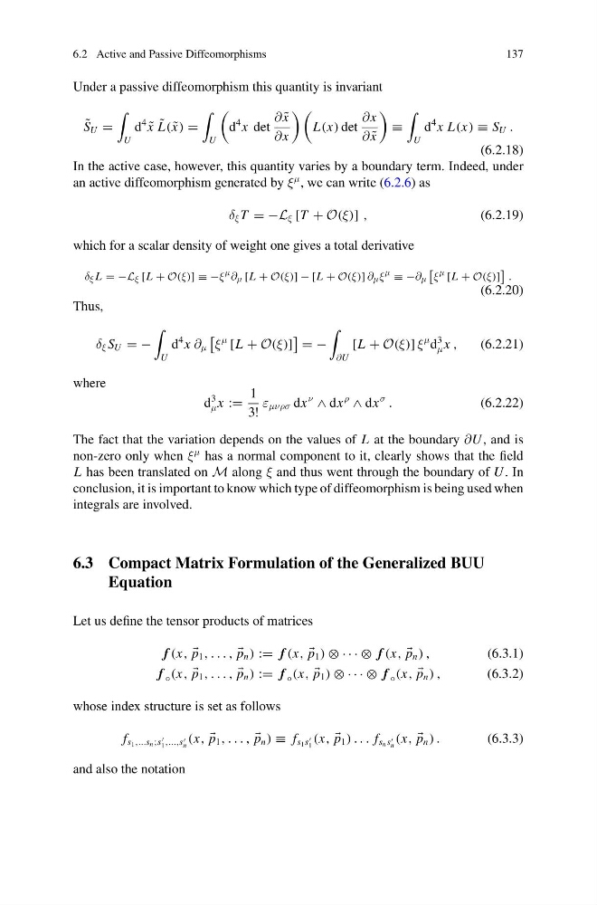
Under a passive diffeomorphism this quantity is invariant
˜
S U =
U
d
4
˜
x ˜
L( ˜
x) =
U
d
4 x det
∂ ˜
x
∂x
L(x) det
∂x
∂ ˜
x
≡
U
d
4 x L(x) ≡ S U .
(6.2.18)
In the active case, however, this quantity varies by a boundary term. Indeed, under
an active diffeomorphism generated by ξ
μ , we can write (6.2.6) as
δ ξ T = −L ξ [T + O(ξ)] ,
(6.2.19)
which for a scalar density of weight one gives a total derivative
δ ξ L = −L ξ [L + O(ξ)] ≡ −ξ
μ ∂ μ [L + O(ξ)] − [L + O(ξ)] ∂ μ ξ
μ ≡ −∂ μ
ξ
μ [L + O(ξ)]
.
(6.2.20)
Thus,
δ ξ S U = −
U
d
4 x ∂ μ
ξ
μ [L + O(ξ)]
= −
∂U
[L + O(ξ)] ξ
μ d
3
μ x ,
(6.2.21)
where
d
3
μ x :=
1
3!
ε μνρσ dx
ν
∧ dx
ρ
∧ dx
σ
.
(6.2.22)
The fact that the variation depends on the values of L at the boundary ∂U , and is
non-zero only when ξ
μ has a normal component to it, clearly shows that the field
L has been translated on M along ξ and thus went through the boundary of U . In
conclusion, it is important to know which type of diffeomorphism is being used when
integrals are involved.
6.3 Compact Matrix Formulation of the Generalized BUU
Equation
Let us define the tensor products of matrices
f (x,
p 1 , . . . ,
p n ) := f (x,
p 1 ) ⊗ · · · ⊗ f (x,
p n ) ,
(6.3.1)
f ◦ (x,
p 1 , . . . ,
p n ) := f ◦ (x,
p 1 ) ⊗ · · · ⊗ f ◦ (x,
p n ) ,
(6.3.2)
whose index structure is set as follows
f s 1 ,...s n ;s
1 ,...,s
n
(x,
p 1 , . . . ,
p n ) ≡ f s 1 s
1
(x,
p 1 ) . . . f s n s
n
(x,
p n ) .
(6.3.3)
and also the notation
137
Under a passive diffeomorphism this quantity is invariant
˜
S U =
U
d
4
˜
x ˜
L( ˜
x) =
U
d
4 x det
∂ ˜
x
∂x
L(x) det
∂x
∂ ˜
x
≡
U
d
4 x L(x) ≡ S U .
(6.2.18)
In the active case, however, this quantity varies by a boundary term. Indeed, under
an active diffeomorphism generated by ξ
μ , we can write (6.2.6) as
δ ξ T = −L ξ [T + O(ξ)] ,
(6.2.19)
which for a scalar density of weight one gives a total derivative
δ ξ L = −L ξ [L + O(ξ)] ≡ −ξ
μ ∂ μ [L + O(ξ)] − [L + O(ξ)] ∂ μ ξ
μ ≡ −∂ μ
ξ
μ [L + O(ξ)]
.
(6.2.20)
Thus,
δ ξ S U = −
U
d
4 x ∂ μ
ξ
μ [L + O(ξ)]
= −
∂U
[L + O(ξ)] ξ
μ d
3
μ x ,
(6.2.21)
where
d
3
μ x :=
1
3!
ε μνρσ dx
ν
∧ dx
ρ
∧ dx
σ
.
(6.2.22)
The fact that the variation depends on the values of L at the boundary ∂U , and is
non-zero only when ξ
μ has a normal component to it, clearly shows that the field
L has been translated on M along ξ and thus went through the boundary of U . In
conclusion, it is important to know which type of diffeomorphism is being used when
integrals are involved.
6.3 Compact Matrix Formulation of the Generalized BUU
Equation
Let us define the tensor products of matrices
f (x,
p 1 , . . . ,
p n ) := f (x,
p 1 ) ⊗ · · · ⊗ f (x,
p n ) ,
(6.3.1)
f ◦ (x,
p 1 , . . . ,
p n ) := f ◦ (x,
p 1 ) ⊗ · · · ⊗ f ◦ (x,
p n ) ,
(6.3.2)
whose index structure is set as follows
f s 1 ,...s n ;s
1 ,...,s
n
(x,
p 1 , . . . ,
p n ) ≡ f s 1 s
1
(x,
p 1 ) . . . f s n s
n
(x,
p n ) .
(6.3.3)
and also the notation