

282
13 Computer-Aided Wind Tunnel Test and Analysis
measured in the flow and the values resulting from the numerical solution of the
Navier–Stokes equations. Thus, this method can be used to improve the quality of
results from PIV measurements, by spatial resolution refinement, extension of the
field explored beyond the field of acquisition and the reconstruction of quantities not
captured from the measurements. In this context, it is also necessary to cite the Proper
Orthogonal Decomposition (POD) method, based on an incomplete decomposition
which was employed successfully to rebuild missing PIV images.
In an unsteady framework, data reconstruction can be also used to carry out a
noise filtering, to improve space and time super-resolution of insufficiently sampled
PIV measurements. Within this framework, either the complete unsteady Navier–
Stokes equations are used, or simplified models less expensive in computing times.
As for the previous example, the optimisation algorithm is obtained by building a set
of differential equations which expresses adequacy between simulated flow and the
whole set of available data (i.e., all images available of the time series over which
the reconstruction applies), with the constraint of respecting the governing equations
chosen for the model. The control variables are normally the boundary and initial
conditions of the simulation.
Such approaches were successfully applied within various frameworks: for
instance in poorly seeded for time-resolved PIV measurements, where the reliability and accuracy of the data relies on tracking a large sample of particles (see
Sect. 11.6.5). In the case of over-seeded PIV measurements, the data reconstruction
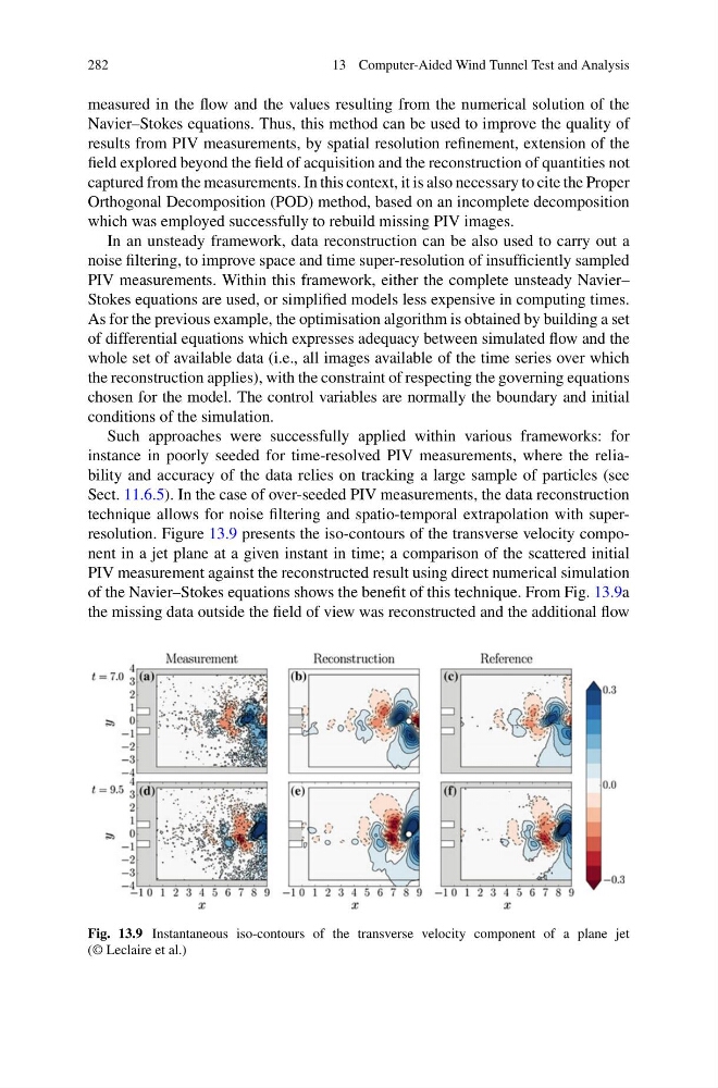
technique allows for noise filtering and spatio-temporal extrapolation with superresolution. Figure 13.9 presents the iso-contours of the transverse velocity component in a jet plane at a given instant in time; a comparison of the scattered initial
PIV measurement against the reconstructed result using direct numerical simulation
of the Navier–Stokes equations shows the benefit of this technique. From Fig. 13.9a
the missing data outside the field of view was reconstructed and the additional flow
Fig. 13.9 Instantaneous iso-contours of the transverse velocity component of a plane jet
(© Leclaire et al.)
13 Computer-Aided Wind Tunnel Test and Analysis
measured in the flow and the values resulting from the numerical solution of the
Navier–Stokes equations. Thus, this method can be used to improve the quality of
results from PIV measurements, by spatial resolution refinement, extension of the
field explored beyond the field of acquisition and the reconstruction of quantities not
captured from the measurements. In this context, it is also necessary to cite the Proper
Orthogonal Decomposition (POD) method, based on an incomplete decomposition
which was employed successfully to rebuild missing PIV images.
In an unsteady framework, data reconstruction can be also used to carry out a
noise filtering, to improve space and time super-resolution of insufficiently sampled
PIV measurements. Within this framework, either the complete unsteady Navier–
Stokes equations are used, or simplified models less expensive in computing times.
As for the previous example, the optimisation algorithm is obtained by building a set
of differential equations which expresses adequacy between simulated flow and the
whole set of available data (i.e., all images available of the time series over which
the reconstruction applies), with the constraint of respecting the governing equations
chosen for the model. The control variables are normally the boundary and initial
conditions of the simulation.
Such approaches were successfully applied within various frameworks: for
instance in poorly seeded for time-resolved PIV measurements, where the reliability and accuracy of the data relies on tracking a large sample of particles (see
Sect. 11.6.5). In the case of over-seeded PIV measurements, the data reconstruction
technique allows for noise filtering and spatio-temporal extrapolation with superresolution. Figure 13.9 presents the iso-contours of the transverse velocity component in a jet plane at a given instant in time; a comparison of the scattered initial
PIV measurement against the reconstructed result using direct numerical simulation
of the Navier–Stokes equations shows the benefit of this technique. From Fig. 13.9a
the missing data outside the field of view was reconstructed and the additional flow
Fig. 13.9 Instantaneous iso-contours of the transverse velocity component of a plane jet
(© Leclaire et al.)