

4 Light-Dressed Spectroscopy of Molecules
97
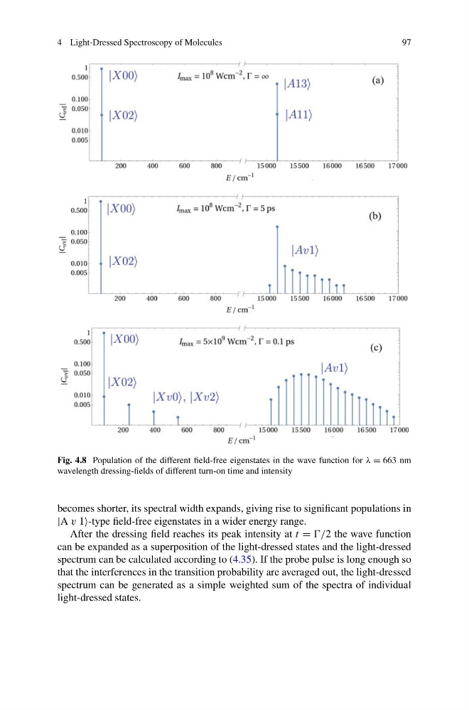
Fig. 4.8 Population of the different field-free eigenstates in the wave function for λ = 663 nm
wavelength dressing-fields of different turn-on time and intensity
becomes shorter, its spectral width expands, giving rise to significant populations in
|A v 1-type field-free eigenstates in a wider energy range.
After the dressing field reaches its peak intensity at t = /2 the wave function
can be expanded as a superposition of the light-dressed states and the light-dressed
spectrum can be calculated according to (4.35). If the probe pulse is long enough so
that the interferences in the transition probability are averaged out, the light-dressed
spectrum can be generated as a simple weighted sum of the spectra of individual
light-dressed states.
97
Fig. 4.8 Population of the different field-free eigenstates in the wave function for λ = 663 nm
wavelength dressing-fields of different turn-on time and intensity
becomes shorter, its spectral width expands, giving rise to significant populations in
|A v 1-type field-free eigenstates in a wider energy range.
After the dressing field reaches its peak intensity at t = /2 the wave function
can be expanded as a superposition of the light-dressed states and the light-dressed
spectrum can be calculated according to (4.35). If the probe pulse is long enough so
that the interferences in the transition probability are averaged out, the light-dressed
spectrum can be generated as a simple weighted sum of the spectra of individual
light-dressed states.