

6.4 Complex Methodology for Reverse Engineering …
557
Overlap region
Overlap region
Overlap region
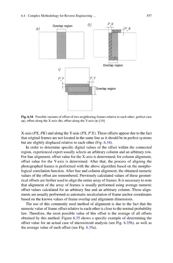
Fig. 6.34 Possible variants of offset of two neighboring frames relative to each other: perfect case
(a); offset along the X-axis (b); offset along the Y-axis (c) [10]
X-axis (PX, PK) and along the Y-axis (PX, P
X). These offsets appear due to the fact
that original frames are not located in the same line as it should be in perfect systems
but are slightly displaced relative to each other (Fig. 6.34).
In order to determine specific digital values of the offset within the connected
region, experienced expert usually selects an arbitrary column and an arbitrary row.
For line alignment, offset value for the X-axis is determined; for column alignment,
offset value for the Y-axis is determined. After that, the process of aligning the
photographed frames is performed with the above algorithm based on the morphological correlation function. After line and column alignment, the obtained numeric
values of the offset are remembered. Previously calculated values of these geometrical offsets are further used to align the entire array of frames. It is necessary to note
that alignment of the array of frames is usually performed using average numeric
offset values calculated for an arbitrary line and an arbitrary column. These alignments are usually performed as automatic recalculation of frame anchor coordinates
based on the known values of frame overlap and alignment dimensions.
The use of this commonly used method of alignment is due to the fact that the
numeric value of frame offset relative to each other is close to the normal probability
law. Therefore, the most possible value of this offset is the average of all offsets
obtained by this method. Figure 6.35 shows a specific example of determining the
offset value for an actual case of microcircuit analysis (see Fig. 6.35b), as well as
the average value of such offset (see Fig. 6.35a).
557
Overlap region
Overlap region
Overlap region
Fig. 6.34 Possible variants of offset of two neighboring frames relative to each other: perfect case
(a); offset along the X-axis (b); offset along the Y-axis (c) [10]
X-axis (PX, PK) and along the Y-axis (PX, P
X). These offsets appear due to the fact
that original frames are not located in the same line as it should be in perfect systems
but are slightly displaced relative to each other (Fig. 6.34).
In order to determine specific digital values of the offset within the connected
region, experienced expert usually selects an arbitrary column and an arbitrary row.
For line alignment, offset value for the X-axis is determined; for column alignment,
offset value for the Y-axis is determined. After that, the process of aligning the
photographed frames is performed with the above algorithm based on the morphological correlation function. After line and column alignment, the obtained numeric
values of the offset are remembered. Previously calculated values of these geometrical offsets are further used to align the entire array of frames. It is necessary to note
that alignment of the array of frames is usually performed using average numeric
offset values calculated for an arbitrary line and an arbitrary column. These alignments are usually performed as automatic recalculation of frame anchor coordinates
based on the known values of frame overlap and alignment dimensions.
The use of this commonly used method of alignment is due to the fact that the
numeric value of frame offset relative to each other is close to the normal probability
law. Therefore, the most possible value of this offset is the average of all offsets
obtained by this method. Figure 6.35 shows a specific example of determining the
offset value for an actual case of microcircuit analysis (see Fig. 6.35b), as well as
the average value of such offset (see Fig. 6.35a).