

402
4 Hardware Trojans in Microcircuits
T (S i−1 ) = p i · 1 + (1 − p i ) · p i · 2 + (1 − p i )
2
· p i · 3 + . . . → ∞
= lim
n→∞
n
j=1
(1 − p i )( j − 1) · p i · j
= lim
n→∞
n
j=1
1 − (1 − p i )
n
p i
− n · (1 − p i )
n
.
(4.1)
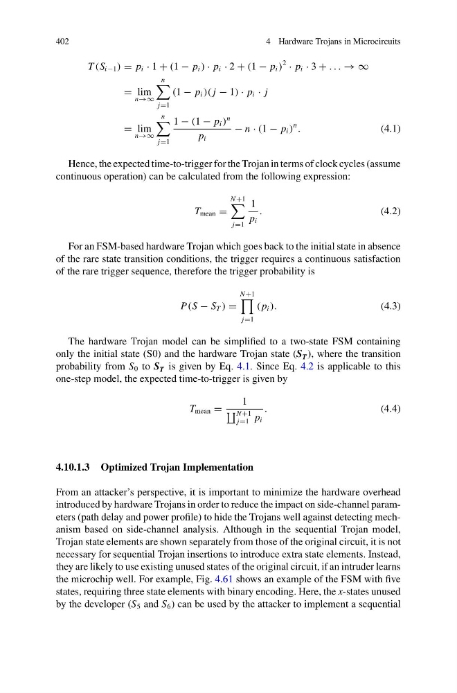
Hence, the expected time-to-trigger for the Trojan in terms of clock cycles (assume
continuous operation) can be calculated from the following expression:
T mean =
N +1
j=1
1
p i
.
(4.2)
For an FSM-based hardware Trojan which goes back to the initial state in absence
of the rare state transition conditions, the trigger requires a continuous satisfaction
of the rare trigger sequence, therefore the trigger probability is
P(S − S T ) =
N +1
j=1
( p i ).
(4.3)
The hardware Trojan model can be simplified to a two-state FSM containing
only the initial state (S0) and the hardware Trojan state (S T ), where the transition
probability from S 0 to S T is given by Eq. 4.1. Since Eq. 4.2 is applicable to this
one-step model, the expected time-to-trigger is given by
T mean =
1
N +1
j=1 p i
.
(4.4)
4.10.1.3 Optimized Trojan Implementation
From an attacker’s perspective, it is important to minimize the hardware overhead
introduced by hardware Trojans in order to reduce the impact on side-channel parameters (path delay and power profile) to hide the Trojans well against detecting mechanism based on side-channel analysis. Although in the sequential Trojan model,
Trojan state elements are shown separately from those of the original circuit, it is not
necessary for sequential Trojan insertions to introduce extra state elements. Instead,
they are likely to use existing unused states of the original circuit, if an intruder learns
the microchip well. For example, Fig. 4.61 shows an example of the FSM with five
states, requiring three state elements with binary encoding. Here, the x-states unused
by the developer (S 5 and S 6 ) can be used by the attacker to implement a sequential
4 Hardware Trojans in Microcircuits
T (S i−1 ) = p i · 1 + (1 − p i ) · p i · 2 + (1 − p i )
2
· p i · 3 + . . . → ∞
= lim
n→∞
n
j=1
(1 − p i )( j − 1) · p i · j
= lim
n→∞
n
j=1
1 − (1 − p i )
n
p i
− n · (1 − p i )
n
.
(4.1)
Hence, the expected time-to-trigger for the Trojan in terms of clock cycles (assume
continuous operation) can be calculated from the following expression:
T mean =
N +1
j=1
1
p i
.
(4.2)
For an FSM-based hardware Trojan which goes back to the initial state in absence
of the rare state transition conditions, the trigger requires a continuous satisfaction
of the rare trigger sequence, therefore the trigger probability is
P(S − S T ) =
N +1
j=1
( p i ).
(4.3)
The hardware Trojan model can be simplified to a two-state FSM containing
only the initial state (S0) and the hardware Trojan state (S T ), where the transition
probability from S 0 to S T is given by Eq. 4.1. Since Eq. 4.2 is applicable to this
one-step model, the expected time-to-trigger is given by
T mean =
1
N +1
j=1 p i
.
(4.4)
4.10.1.3 Optimized Trojan Implementation
From an attacker’s perspective, it is important to minimize the hardware overhead
introduced by hardware Trojans in order to reduce the impact on side-channel parameters (path delay and power profile) to hide the Trojans well against detecting mechanism based on side-channel analysis. Although in the sequential Trojan model,
Trojan state elements are shown separately from those of the original circuit, it is not
necessary for sequential Trojan insertions to introduce extra state elements. Instead,
they are likely to use existing unused states of the original circuit, if an intruder learns
the microchip well. For example, Fig. 4.61 shows an example of the FSM with five
states, requiring three state elements with binary encoding. Here, the x-states unused
by the developer (S 5 and S 6 ) can be used by the attacker to implement a sequential