

Automated Upgraded Generalized Full-Discretization Method …
87
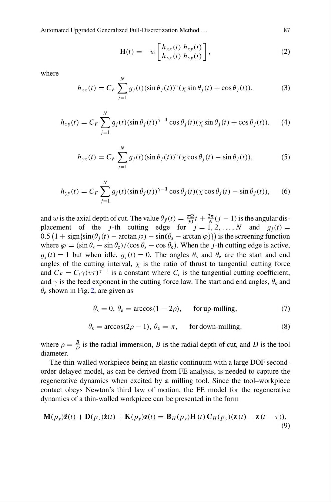
H(t) = −w
h xx (t) h xy (t)
h yx (t) h yy (t)
,
(2)
where
h xx (t) = C F
N
j=1
g j (t)(sin θ j (t))
γ
(χ sin θ j (t) + cos θ j (t)),
(3)
h xy (t) = C F
N
j=1
g j (t)(sin θ j (t))
γ−1 cos θ j (t)(χ sin θ j (t) + cos θ j (t)), (4)
h yx (t) = C F
N
j=1
g j (t)(sin θ j (t))
γ
(χ cos θ j (t) − sin θ j (t)),
(5)
h yy (t) = C F
N
j=1
g j (t)(sin θ j (t))
γ−1 cos θ j (t)(χ cos θ j (t) − sin θ j (t)), (6)
and w is the axial depth of cut. The value θ j (t) =
π
30
t +
2π
N
( j − 1) is the angular displacement of the j-th cutting edge for j = 1, 2, . . . , N and g j (t) =
0.5
1 + sign{sin(θ j (t) − arctan ℘) − sin(θ s − arctan ℘)}
is the screening function
where ℘ = (sin θ s − sin θ e )/(cos θ s − cos θ e ). When the j-th cutting edge is active,
g j (t) = 1 but when idle, g j (t) = 0. The angles θ s and θ e are the start and end
angles of the cutting interval, χ is the ratio of thrust to tangential cutting force
and C F = C t γ(vτ )
γ−1 is a constant where C t is the tangential cutting coefficient,
and γ is the feed exponent in the cutting force law. The start and end angles, θ s and
θ e shown in Fig. 2, are given as
θ s = 0, θ e = arccos(1 − 2ρ),
for up-milling,
(7)
θ s = arccos(2ρ − 1), θ e = π,
for down-milling,
(8)
where ρ =
B
D
is the radial immersion, B is the radial depth of cut, and D is the tool
diameter.
The thin-walled workpiece being an elastic continuum with a large DOF secondorder delayed model, as can be derived from FE analysis, is needed to capture the
regenerative dynamics when excited by a milling tool. Since the tool–workpiece
contact obeys Newton’s third law of motion, the FE model for the regenerative
dynamics of a thin-walled workpiece can be presented in the form
M( p y )¨ z(t) + D( p y )˙ z(t) + K( p y )z(t) = B H ( p y )H (t) C H ( p y )(z (t) − z (t − τ )),
(9)
87
H(t) = −w
h xx (t) h xy (t)
h yx (t) h yy (t)
,
(2)
where
h xx (t) = C F
N
j=1
g j (t)(sin θ j (t))
γ
(χ sin θ j (t) + cos θ j (t)),
(3)
h xy (t) = C F
N
j=1
g j (t)(sin θ j (t))
γ−1 cos θ j (t)(χ sin θ j (t) + cos θ j (t)), (4)
h yx (t) = C F
N
j=1
g j (t)(sin θ j (t))
γ
(χ cos θ j (t) − sin θ j (t)),
(5)
h yy (t) = C F
N
j=1
g j (t)(sin θ j (t))
γ−1 cos θ j (t)(χ cos θ j (t) − sin θ j (t)), (6)
and w is the axial depth of cut. The value θ j (t) =
π
30
t +
2π
N
( j − 1) is the angular displacement of the j-th cutting edge for j = 1, 2, . . . , N and g j (t) =
0.5
1 + sign{sin(θ j (t) − arctan ℘) − sin(θ s − arctan ℘)}
is the screening function
where ℘ = (sin θ s − sin θ e )/(cos θ s − cos θ e ). When the j-th cutting edge is active,
g j (t) = 1 but when idle, g j (t) = 0. The angles θ s and θ e are the start and end
angles of the cutting interval, χ is the ratio of thrust to tangential cutting force
and C F = C t γ(vτ )
γ−1 is a constant where C t is the tangential cutting coefficient,
and γ is the feed exponent in the cutting force law. The start and end angles, θ s and
θ e shown in Fig. 2, are given as
θ s = 0, θ e = arccos(1 − 2ρ),
for up-milling,
(7)
θ s = arccos(2ρ − 1), θ e = π,
for down-milling,
(8)
where ρ =
B
D
is the radial immersion, B is the radial depth of cut, and D is the tool
diameter.
The thin-walled workpiece being an elastic continuum with a large DOF secondorder delayed model, as can be derived from FE analysis, is needed to capture the
regenerative dynamics when excited by a milling tool. Since the tool–workpiece
contact obeys Newton’s third law of motion, the FE model for the regenerative
dynamics of a thin-walled workpiece can be presented in the form
M( p y )¨ z(t) + D( p y )˙ z(t) + K( p y )z(t) = B H ( p y )H (t) C H ( p y )(z (t) − z (t − τ )),
(9)