

444
M. N. Bojnordi and P. Behnam
>
Z 11 Z 12
Z 14
Z 13
N/2
...
Channel 1
Channel 3
...
Step 1
Step 2
X 11 X 12
X 14 X 15
X 13
X 16
X 17 X 18 X 19
F 11 F 12
F 14
F 13
Y 11 = X 11 F 11 + X 12 F 12
+ X 14 F 13 + X 14 F 14
X 31 X 32
X 34 X 35
X 33
X 36
X 37 X 38 X 39
F 31 F 32
F 34
F 33
Y 31 = X 31 F 31 + X 32 F 32
+ X 34 F 33 + X 34 F 34
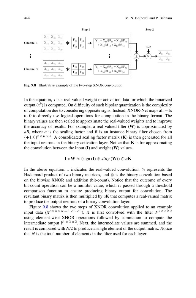
Fig. 9.8 Illustrative example of the two-step XNOR convolution
In the equation, x is a real-valued weight or activation data for which the binarized
output (x b ) is computed. On difficulty of such bipolar quantization is the complexity
of computation due to considering opposite signs. Instead, XNOR-Net maps all −1s
to 0 to directly use logical operations for computation in the binary format. The
binary values are then scaled to approximate the real-valued weights and to improve
the accuracy of results. For example, a real-valued filter (W) is approximated by
aB, where a is the scaling factor and B is an instance binary filter chosen from
{+1, 0} x × w × h . A consolidated scaling factor matrix (K) is then generated for all
the input neurons in the binary activation layer. Notice that K is for approximating
the convolution between the input (I) and weight (W) values.
I ∗ W ≈ (sign (I) sing (W)) aK
In the above equation, ∗ indicates the real-valued convolution, represents the
Hadamard product of two binary matrices, and is the binary convolution based
on the bitwise XNOR and addition (bit-count). Notice that the outcome of every
bit-count operation can be a multibit value, which is passed through a threshold
comparison function to ensure producing binary output for convolution. The
resultant binary matrix is then multiplied by aK that computes a real-valued matrix
to produce the output neurons of a binary convolution layer.
Figure 9.8 shows the two steps of XNOR convolution applied to an example
input data (X c × h × w = 3 × 3 × 3 ). X is first convolved with the filter F 3 × 2 × 2
using element-wise XNOR operations followed by summation to compute the
intermediate output Y 1 × 2 × 2 . Next, the intermediate values are summed, and the
result is compared with N/2 to produce a single element of the output matrix. Notice
that N is the total number of elements in the filter used for each layer.
M. N. Bojnordi and P. Behnam
>
Z 11 Z 12
Z 14
Z 13
N/2
...
Channel 1
Channel 3
...
Step 1
Step 2
X 11 X 12
X 14 X 15
X 13
X 16
X 17 X 18 X 19
F 11 F 12
F 14
F 13
Y 11 = X 11 F 11 + X 12 F 12
+ X 14 F 13 + X 14 F 14
X 31 X 32
X 34 X 35
X 33
X 36
X 37 X 38 X 39
F 31 F 32
F 34
F 33
Y 31 = X 31 F 31 + X 32 F 32
+ X 34 F 33 + X 34 F 34
Fig. 9.8 Illustrative example of the two-step XNOR convolution
In the equation, x is a real-valued weight or activation data for which the binarized
output (x b ) is computed. On difficulty of such bipolar quantization is the complexity
of computation due to considering opposite signs. Instead, XNOR-Net maps all −1s
to 0 to directly use logical operations for computation in the binary format. The
binary values are then scaled to approximate the real-valued weights and to improve
the accuracy of results. For example, a real-valued filter (W) is approximated by
aB, where a is the scaling factor and B is an instance binary filter chosen from
{+1, 0} x × w × h . A consolidated scaling factor matrix (K) is then generated for all
the input neurons in the binary activation layer. Notice that K is for approximating
the convolution between the input (I) and weight (W) values.
I ∗ W ≈ (sign (I) sing (W)) aK
In the above equation, ∗ indicates the real-valued convolution, represents the
Hadamard product of two binary matrices, and is the binary convolution based
on the bitwise XNOR and addition (bit-count). Notice that the outcome of every
bit-count operation can be a multibit value, which is passed through a threshold
comparison function to ensure producing binary output for convolution. The
resultant binary matrix is then multiplied by aK that computes a real-valued matrix
to produce the output neurons of a binary convolution layer.
Figure 9.8 shows the two steps of XNOR convolution applied to an example
input data (X c × h × w = 3 × 3 × 3 ). X is first convolved with the filter F 3 × 2 × 2
using element-wise XNOR operations followed by summation to compute the
intermediate output Y 1 × 2 × 2 . Next, the intermediate values are summed, and the
result is compared with N/2 to produce a single element of the output matrix. Notice
that N is the total number of elements in the filter used for each layer.