

290
F. Firouzi et al.
f
1
0
f2
0
Decision
boundary
4
6
2
6
4
2
f2 < 3
f1 < 4
f1 < 3
f2 < 5
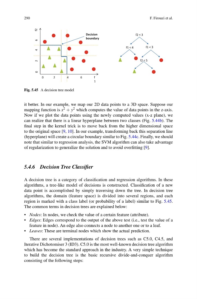
Fig. 5.45 A decision tree model
it better. In our example, we map our 2D data points to a 3D space. Suppose our
mapping function is x 2 + y 2 which computes the value of data points in the z-axis.
Now if we plot the data points using the newly computed values (x-z plane), we
can realize that there is a linear hyperplane between two classes (Fig. 5.44b). The
final step in the kernel trick is to move back from the higher dimensional space
to the original space [9, 10]. In our example, transforming back this separation line
(hyperplane) will create a circular boundary similar to Fig. 5.44c. Finally, we should
note that similar to regression analysis, the SVM algorithm can also take advantage
of regularization to generalize the solution and to avoid overfitting [9].
5.4.6 Decision Tree Classifier
A decision tree is a category of classification and regression algorithms. In these
algorithms, a tree-like model of decisions is constructed. Classification of a new
data point is accomplished by simply traversing down the tree. In decision tree
algorithms, the domain (feature space) is divided into several regions, and each
region is marked with a class label (or probability of a label) similar to Fig. 5.45.
The common terms in decision trees are explained below:
• Nodes: In nodes, we check the value of a certain feature (attribute).
• Edges: Edges correspond to the output of the above test (i.e., test the value of a
feature in node). An edge also connects a node to another one or to a leaf.
• Leaves: These are terminal nodes which show the actual prediction.
There are several implementations of decision trees such as C5.0, C4.5, and
Iterative Dichotomiser 3 (ID3). C5.0 is the most well-known decision tree algorithm
which has become the standard approach in the industry. A very simple technique
to build the decision tree is the basic recursive divide-and-conquer algorithm
consisting of the following steps:
F. Firouzi et al.
f
1
0
f2
0
Decision
boundary
4
6
2
6
4
2
f2 < 3
f1 < 4
f1 < 3
f2 < 5
Fig. 5.45 A decision tree model
it better. In our example, we map our 2D data points to a 3D space. Suppose our
mapping function is x 2 + y 2 which computes the value of data points in the z-axis.
Now if we plot the data points using the newly computed values (x-z plane), we
can realize that there is a linear hyperplane between two classes (Fig. 5.44b). The
final step in the kernel trick is to move back from the higher dimensional space
to the original space [9, 10]. In our example, transforming back this separation line
(hyperplane) will create a circular boundary similar to Fig. 5.44c. Finally, we should
note that similar to regression analysis, the SVM algorithm can also take advantage
of regularization to generalize the solution and to avoid overfitting [9].
5.4.6 Decision Tree Classifier
A decision tree is a category of classification and regression algorithms. In these
algorithms, a tree-like model of decisions is constructed. Classification of a new
data point is accomplished by simply traversing down the tree. In decision tree
algorithms, the domain (feature space) is divided into several regions, and each
region is marked with a class label (or probability of a label) similar to Fig. 5.45.
The common terms in decision trees are explained below:
• Nodes: In nodes, we check the value of a certain feature (attribute).
• Edges: Edges correspond to the output of the above test (i.e., test the value of a
feature in node). An edge also connects a node to another one or to a leaf.
• Leaves: These are terminal nodes which show the actual prediction.
There are several implementations of decision trees such as C5.0, C4.5, and
Iterative Dichotomiser 3 (ID3). C5.0 is the most well-known decision tree algorithm
which has become the standard approach in the industry. A very simple technique
to build the decision tree is the basic recursive divide-and-conquer algorithm
consisting of the following steps: