

5 Machine Learning for IoT
267
W 1
W 2
L1 norm
W 2
L2 norm
W 1
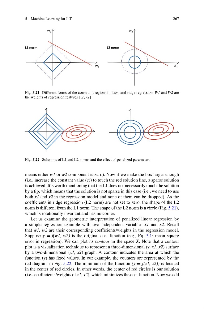
Fig. 5.21 Different forms of the constraint regions in lasso and ridge regression. W1 and W2 are
the weights of regression features [x1, x2]
Fig. 5.22 Solutions of L1 and L2 norms and the effect of penalized parameters
means either w1 or w2 component is zero). Now if we make the box larger enough
(i.e., increase the constant value (c)) to touch the red solution line, a sparse solution
is achieved. It’s worth mentioning that the L1 does not necessarily touch the solution
by a tip, which means that the solution is not sparse in this case (i.e., we need to use
both x1 and x2 in the regression model and none of them can be dropped). As the
coefficients in ridge regression (L2 norm) are not set to zero, the shape of the L2
norm is different from the L1 norm. The shape of the L2 norm is a circle (Fig. 5.21),
which is rotationally invariant and has no corner.
Let us examine the geometric interpretation of penalized linear regression by
a simple regression example with two independent variables x1 and x2. Recall
that w1, w2 are their corresponding coefficients/weights in the regression model.
Suppose y = f(w1, w2) is the original cost function (e.g., Eq. 5.1: mean square
error in regression). We can plot its contour in the space X. Note that a contour
plot is a visualization technique to represent a three-dimensional (y, x1, x2) surface
by a two-dimensional (x1, x2) graph. A contour indicates the area at which the
function (y) has fixed values. In our example, the counters are represented by the
red diagram in Fig. 5.22. The minimum of the function (y = f(x1, x2)) is located
in the center of red circles. In other words, the center of red circles is our solution
(i.e., coefficients/weights of x1, x2), which minimizes the cost function. Now we add
267
W 1
W 2
L1 norm
W 2
L2 norm
W 1
Fig. 5.21 Different forms of the constraint regions in lasso and ridge regression. W1 and W2 are
the weights of regression features [x1, x2]
Fig. 5.22 Solutions of L1 and L2 norms and the effect of penalized parameters
means either w1 or w2 component is zero). Now if we make the box larger enough
(i.e., increase the constant value (c)) to touch the red solution line, a sparse solution
is achieved. It’s worth mentioning that the L1 does not necessarily touch the solution
by a tip, which means that the solution is not sparse in this case (i.e., we need to use
both x1 and x2 in the regression model and none of them can be dropped). As the
coefficients in ridge regression (L2 norm) are not set to zero, the shape of the L2
norm is different from the L1 norm. The shape of the L2 norm is a circle (Fig. 5.21),
which is rotationally invariant and has no corner.
Let us examine the geometric interpretation of penalized linear regression by
a simple regression example with two independent variables x1 and x2. Recall
that w1, w2 are their corresponding coefficients/weights in the regression model.
Suppose y = f(w1, w2) is the original cost function (e.g., Eq. 5.1: mean square
error in regression). We can plot its contour in the space X. Note that a contour
plot is a visualization technique to represent a three-dimensional (y, x1, x2) surface
by a two-dimensional (x1, x2) graph. A contour indicates the area at which the
function (y) has fixed values. In our example, the counters are represented by the
red diagram in Fig. 5.22. The minimum of the function (y = f(x1, x2)) is located
in the center of red circles. In other words, the center of red circles is our solution
(i.e., coefficients/weights of x1, x2), which minimizes the cost function. Now we add