

5 Machine Learning for IoT
251
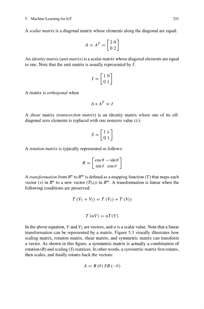
A scalar matrix is a diagonal matrix whose elements along the diagonal are equal:
A = A
T
=
2 0
0 2
An identity matrix (unit matrix) is a scalar matrix whose diagonal elements are equal
to one. Note that the unit matrix is usually represented by I:
I =
1 0
0 1
A matrix is orthogonal when
A ∗ A
T
= I
A shear matrix (transvection matrix) is an identity matrix where one of its offdiagonal zero elements is replaced with one nonzero value (λ):
S =
1 λ
0 1
A rotation matrix is typically represented as follows:
R =
cos θ − sin θ
sin θ cos θ
A transformation from R n to R m is defined as a mapping function (T) that maps each
vector (x) in R n to a new vector (T(x)) in R m . A transformation is linear when the
following conditions are preserved:
T (V 1 + V 2 ) = T (V 1 ) + T (V 2 )
T (αV ) = αT (V )
In the above equation, V and V 2 are vectors, and α is a scalar value. Note that a linear
transformation can be represented by a matrix. Figure 5.3 visually illustrates how
scaling matrix, rotation matrix, shear matrix, and symmetric matrix can transform
a vector. As shown in this figure, a symmetric matrix is actually a combination of
rotation (R) and scaling (S) matrices. In other words, a symmetric matrix first rotates,
then scales, and finally rotates back the vectors:
A = R (θ ) SR (−θ )
251
A scalar matrix is a diagonal matrix whose elements along the diagonal are equal:
A = A
T
=
2 0
0 2
An identity matrix (unit matrix) is a scalar matrix whose diagonal elements are equal
to one. Note that the unit matrix is usually represented by I:
I =
1 0
0 1
A matrix is orthogonal when
A ∗ A
T
= I
A shear matrix (transvection matrix) is an identity matrix where one of its offdiagonal zero elements is replaced with one nonzero value (λ):
S =
1 λ
0 1
A rotation matrix is typically represented as follows:
R =
cos θ − sin θ
sin θ cos θ
A transformation from R n to R m is defined as a mapping function (T) that maps each
vector (x) in R n to a new vector (T(x)) in R m . A transformation is linear when the
following conditions are preserved:
T (V 1 + V 2 ) = T (V 1 ) + T (V 2 )
T (αV ) = αT (V )
In the above equation, V and V 2 are vectors, and α is a scalar value. Note that a linear
transformation can be represented by a matrix. Figure 5.3 visually illustrates how
scaling matrix, rotation matrix, shear matrix, and symmetric matrix can transform
a vector. As shown in this figure, a symmetric matrix is actually a combination of
rotation (R) and scaling (S) matrices. In other words, a symmetric matrix first rotates,
then scales, and finally rotates back the vectors:
A = R (θ ) SR (−θ )