

58
4 Dimensioning Droplet Microfluidic Networks
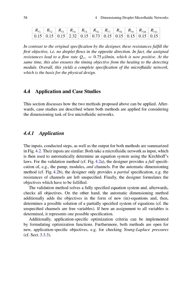
R c 1 R c 2 R c 3 R c 4 R c 5 R c 6 R c 7 R c 8 R c 9 R c 10 R c 11
0.15 0.15 0.15 2.32 0.15 0.73 0.15 0.15 0.15 0.15 0.15
In contrast to the original specification by the designer, these resistances fulfill the
first objective, i.e. no droplet flows in the opposite direction. In fact, the assigned
resistances lead to a flow rate Q c 7 = 0.75 μl/min, which is now positive. At the
same time, this also ensures the timing objective from the heating to the detecting
module. Overall, this yields a complete specification of the microfluidic network,
which is the basis for the physical design.
4.4 Application and Case Studies
This section discusses how the two methods proposed above can be applied. Afterwards, case studies are described where both methods are applied for considering
the dimensioning task of five microfluidic networks.
4.4.1 Application
The inputs, conducted steps, as well as the output for both methods are summarized
in Fig. 4.2. Their inputs are similar: Both take a microfluidic network as input, which
is then used to automatically determine an equation system using the Kirchhoff’s
laws. For the validation method (cf. Fig. 4.2a), the designer provides a full specification of, e.g., the pump, modules, and channels. For the automatic dimensioning
method (cf. Fig. 4.2b), the designer only provides a partial specification, e.g. the
resistances of channels are left unspecified. Finally, the designer formulates the
objectives which have to be fulfilled.
The validation method solves a fully specified equation system and, afterwards,
checks all objectives. On the other hand, the automatic dimensioning method
additionally adds the objectives in the form of new (in)-equations and, then,
determines a possible solution of a partially specified system of equations (cf. the
unspecified channels are free variables). If here an assignment to all variables is
determined, it represents one possible specification.
Additionally, application-specific optimization criteria can be implemented
by formulating optimization functions. Furthermore, both methods are open for
new, application-specific objectives, e.g. for checking Young-Laplace pressures
(cf. Sect. 3.3.3).
4 Dimensioning Droplet Microfluidic Networks
R c 1 R c 2 R c 3 R c 4 R c 5 R c 6 R c 7 R c 8 R c 9 R c 10 R c 11
0.15 0.15 0.15 2.32 0.15 0.73 0.15 0.15 0.15 0.15 0.15
In contrast to the original specification by the designer, these resistances fulfill the
first objective, i.e. no droplet flows in the opposite direction. In fact, the assigned
resistances lead to a flow rate Q c 7 = 0.75 μl/min, which is now positive. At the
same time, this also ensures the timing objective from the heating to the detecting
module. Overall, this yields a complete specification of the microfluidic network,
which is the basis for the physical design.
4.4 Application and Case Studies
This section discusses how the two methods proposed above can be applied. Afterwards, case studies are described where both methods are applied for considering
the dimensioning task of five microfluidic networks.
4.4.1 Application
The inputs, conducted steps, as well as the output for both methods are summarized
in Fig. 4.2. Their inputs are similar: Both take a microfluidic network as input, which
is then used to automatically determine an equation system using the Kirchhoff’s
laws. For the validation method (cf. Fig. 4.2a), the designer provides a full specification of, e.g., the pump, modules, and channels. For the automatic dimensioning
method (cf. Fig. 4.2b), the designer only provides a partial specification, e.g. the
resistances of channels are left unspecified. Finally, the designer formulates the
objectives which have to be fulfilled.
The validation method solves a fully specified equation system and, afterwards,
checks all objectives. On the other hand, the automatic dimensioning method
additionally adds the objectives in the form of new (in)-equations and, then,
determines a possible solution of a partially specified system of equations (cf. the
unspecified channels are free variables). If here an assignment to all variables is
determined, it represents one possible specification.
Additionally, application-specific optimization criteria can be implemented
by formulating optimization functions. Furthermore, both methods are open for
new, application-specific objectives, e.g. for checking Young-Laplace pressures
(cf. Sect. 3.3.3).