

314
29 Tachyons of Plastic Deformation
= −
2 σa 2
L 2
o κ 2
2+
u 2
c 2
o
− 1
exp
−2
π(x − ut)
L o κ
1+exp
−2
π(x − ut)
L o κ
2 −
σa 2
2L 2
o
1−exp
−2
π(x − ut)
L o κ
2
1+exp
−2
π(x − ut)
L o κ
2
= −
4 σa 2
L 2
o κ 2
exp
−2
π(x − ut)
L o κ
1 + exp
−2
π(x − ut)
L o κ
2 −
σa 2
2L 2
o
1 + exp
−2
π(x − ut)
L o κ
2
1 + exp
−2
π(x − ut)
L o κ
2
= −
1
κ 2
4 σa 2
L 2
o
exp
−2
π(x − ut)
L o κ
1 + exp
−2
π(x − ut)
L o κ
2 −
σa 2
2L 2
o
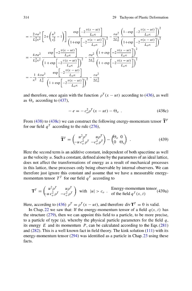
and therefore, once again with the function ρ
T
(x − ut) according to (436), as well
as o according to (437),
− e = − c
2
o ρ
T
(x − ut) − o .
(438c)
From (438) to (438c) we can construct the following energy-momentum tensor T
T
for our field q
T according to the rule (276),
T
T
=
u
2
ρ
T
uρ
T
−u c
2
o ρ
T
−c
2
o ρ
T
−
o 0
0 o
.
(439)
Here the second term is an additive constant, independent of both spacetime as well
as the velocity u. Such a constant, defined alone by the parameters of an ideal lattice,
does not affect the transformations of energy as a result of mechanical processes
in this lattice, these processes only being observable by internal observers. We can
therefore just ignore this constant and assume that we have a measurable energymomentum tensor T
T for our field q
T according to
T
T
=
u
2
ρ
T
uρ
T
−u c
2
o ρ
T
−c
2
o ρ
T
with |u| > c o .
Energy-momentum tensor
of the field q
T
(x, t)
(439a)
Here, according to (436) ρ
T
= ρ
T
(x − ut), and therefore div T
T
= 0 is valid.
In Chap. 22 we saw that: If the energy-momentum tensor of a field q(x, t) has
the structure (279), then we can appoint this field to a particle, to be more precise,
to a particle of type (a), whereby the physical particle parameters for the field q,
its energy E and its momentum P, can be calculated according to the Eqs. (281)
and (282). This is a well known fact in field theory. The kink solution (111) with its
energy-momentum tensor (294) was identified as a particle in Chap. 23 using these
facts.
29 Tachyons of Plastic Deformation
= −
2 σa 2
L 2
o κ 2
2+
u 2
c 2
o
− 1
exp
−2
π(x − ut)
L o κ
1+exp
−2
π(x − ut)
L o κ
2 −
σa 2
2L 2
o
1−exp
−2
π(x − ut)
L o κ
2
1+exp
−2
π(x − ut)
L o κ
2
= −
4 σa 2
L 2
o κ 2
exp
−2
π(x − ut)
L o κ
1 + exp
−2
π(x − ut)
L o κ
2 −
σa 2
2L 2
o
1 + exp
−2
π(x − ut)
L o κ
2
1 + exp
−2
π(x − ut)
L o κ
2
= −
1
κ 2
4 σa 2
L 2
o
exp
−2
π(x − ut)
L o κ
1 + exp
−2
π(x − ut)
L o κ
2 −
σa 2
2L 2
o
and therefore, once again with the function ρ
T
(x − ut) according to (436), as well
as o according to (437),
− e = − c
2
o ρ
T
(x − ut) − o .
(438c)
From (438) to (438c) we can construct the following energy-momentum tensor T
T
for our field q
T according to the rule (276),
T
T
=
u
2
ρ
T
uρ
T
−u c
2
o ρ
T
−c
2
o ρ
T
−
o 0
0 o
.
(439)
Here the second term is an additive constant, independent of both spacetime as well
as the velocity u. Such a constant, defined alone by the parameters of an ideal lattice,
does not affect the transformations of energy as a result of mechanical processes
in this lattice, these processes only being observable by internal observers. We can
therefore just ignore this constant and assume that we have a measurable energymomentum tensor T
T for our field q
T according to
T
T
=
u
2
ρ
T
uρ
T
−u c
2
o ρ
T
−c
2
o ρ
T
with |u| > c o .
Energy-momentum tensor
of the field q
T
(x, t)
(439a)
Here, according to (436) ρ
T
= ρ
T
(x − ut), and therefore div T
T
= 0 is valid.
In Chap. 22 we saw that: If the energy-momentum tensor of a field q(x, t) has
the structure (279), then we can appoint this field to a particle, to be more precise,
to a particle of type (a), whereby the physical particle parameters for the field q,
its energy E and its momentum P, can be calculated according to the Eqs. (281)
and (282). This is a well known fact in field theory. The kink solution (111) with its
energy-momentum tensor (294) was identified as a particle in Chap. 23 using these
facts.