

294
27 The Separation of Eigen Stresses
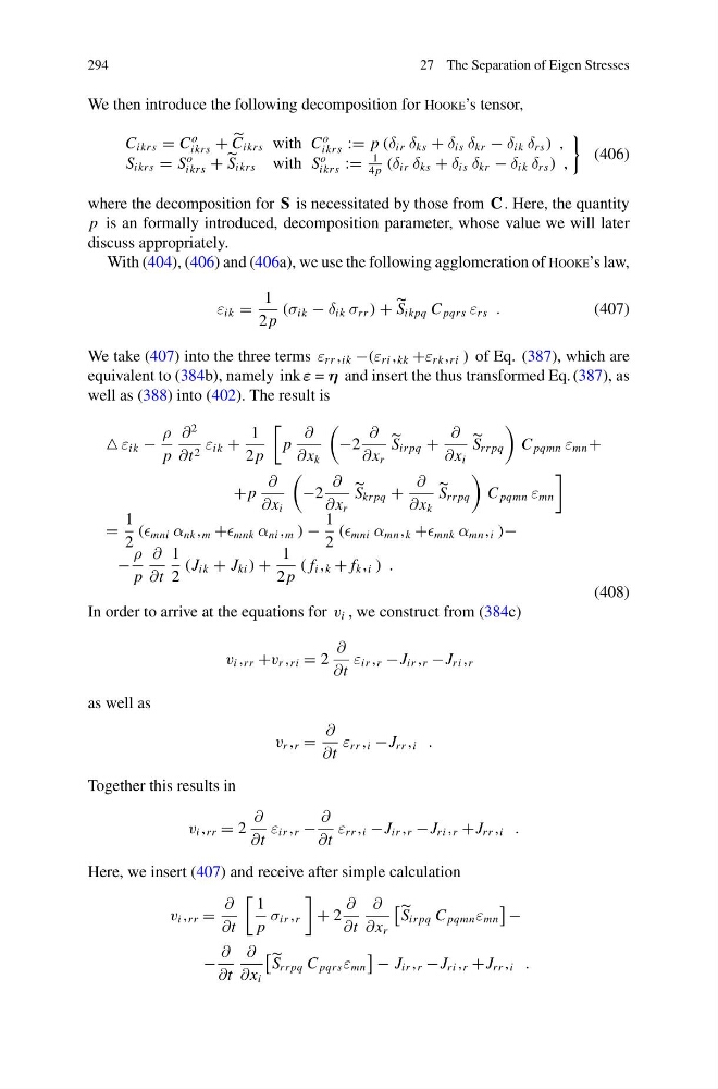
We then introduce the following decomposition for Hooke’s tensor,
C ikrs = C
o
ikrs +
C ikrs with C
o
ikrs := p (δ ir δ ks + δ is δ kr − δ ik δ rs ) ,
S ikrs = S
o
ikrs + S ikrs with S
o
ikrs :=
1
4 p
(δ ir δ ks + δ is δ kr − δ ik δ rs ) ,
(406)
where the decomposition for S is necessitated by those from C . Here, the quantity
p is an formally introduced, decomposition parameter, whose value we will later
discuss appropriately.
With (404), (406) and (406a), we use the following agglomeration of Hooke’s law,
ε ik =
1
2 p
(σ ik − δ ik σ rr ) + S ikpq C pqrs ε rs .
(407)
We take (407) into the three terms ε rr , ik −(ε ri , kk +ε rk , ri ) of Eq. (387), which are
equivalent to (384b), namely ink ε = η and insert the thus transformed Eq. (387), as
well as (388) into (402). The result is
ε ik −
ρ
p
∂
2
∂t 2 ε ik +
1
2 p
p
∂
∂x k
−2
∂
∂x r
S ir pq +
∂
∂x i
S rr pq
C pqmn ε mn +
+ p
∂
∂x i
−2
∂
∂x r
S kr pq +
∂
∂x k
S rr pq
C pqmn ε mn
=
1
2
( mni α nk , m + mnk α ni , m ) −
1
2
( mni α mn , k + mnk α mn , i )−
−
ρ
p
∂
∂t
1
2
(J ik + J ki ) +
1
2 p
( f i , k + f k , i ) .
(408)
In order to arrive at the equations for v i , we construct from (384c)
v i , rr +v r , ri = 2
∂
∂t
ε ir , r −J ir , r −J ri , r
as well as
v r , r =
∂
∂t
ε rr , i −J rr , i .
Together this results in
v i , rr = 2
∂
∂t
ε ir , r −
∂
∂t
ε rr , i −J ir , r −J ri , r +J rr , i .
Here, we insert (407) and receive after simple calculation
v i , rr =
∂
∂t
1
p
σ ir , r
+ 2
∂
∂t
∂
∂x r
S ir pq C pqmn ε mn
−
−
∂
∂t
∂
∂x i
S rr pq C pqrs ε mn
− J ir , r −J ri , r +J rr , i .
27 The Separation of Eigen Stresses
We then introduce the following decomposition for Hooke’s tensor,
C ikrs = C
o
ikrs +
C ikrs with C
o
ikrs := p (δ ir δ ks + δ is δ kr − δ ik δ rs ) ,
S ikrs = S
o
ikrs + S ikrs with S
o
ikrs :=
1
4 p
(δ ir δ ks + δ is δ kr − δ ik δ rs ) ,
(406)
where the decomposition for S is necessitated by those from C . Here, the quantity
p is an formally introduced, decomposition parameter, whose value we will later
discuss appropriately.
With (404), (406) and (406a), we use the following agglomeration of Hooke’s law,
ε ik =
1
2 p
(σ ik − δ ik σ rr ) + S ikpq C pqrs ε rs .
(407)
We take (407) into the three terms ε rr , ik −(ε ri , kk +ε rk , ri ) of Eq. (387), which are
equivalent to (384b), namely ink ε = η and insert the thus transformed Eq. (387), as
well as (388) into (402). The result is
ε ik −
ρ
p
∂
2
∂t 2 ε ik +
1
2 p
p
∂
∂x k
−2
∂
∂x r
S ir pq +
∂
∂x i
S rr pq
C pqmn ε mn +
+ p
∂
∂x i
−2
∂
∂x r
S kr pq +
∂
∂x k
S rr pq
C pqmn ε mn
=
1
2
( mni α nk , m + mnk α ni , m ) −
1
2
( mni α mn , k + mnk α mn , i )−
−
ρ
p
∂
∂t
1
2
(J ik + J ki ) +
1
2 p
( f i , k + f k , i ) .
(408)
In order to arrive at the equations for v i , we construct from (384c)
v i , rr +v r , ri = 2
∂
∂t
ε ir , r −J ir , r −J ri , r
as well as
v r , r =
∂
∂t
ε rr , i −J rr , i .
Together this results in
v i , rr = 2
∂
∂t
ε ir , r −
∂
∂t
ε rr , i −J ir , r −J ri , r +J rr , i .
Here, we insert (407) and receive after simple calculation
v i , rr =
∂
∂t
1
p
σ ir , r
+ 2
∂
∂t
∂
∂x r
S ir pq C pqmn ε mn
−
−
∂
∂t
∂
∂x i
S rr pq C pqrs ε mn
− J ir , r −J ri , r +J rr , i .