

10 Measuring-Rods and Clocks in Motion
99
which is exactly what we wanted to prove.
We will now turn to the clock. Again, the clock moved at the uniform velocity
v has to develop out of the displayed function q
III
o (x, t) in Figs. 9.3 and 9.4 by
a displacement v t to the right, with the important condition that the sine-Gordon
equation maintains its validity. If one simply displaces the function q
III
o (x, t) by v t
to the right, we get according to (105) the function
˜
q
III
o (x, t) =
2a
π
arctan
sin(2πt/T o )
cosh
π(x−vt)
L o
√
2
.
(116)
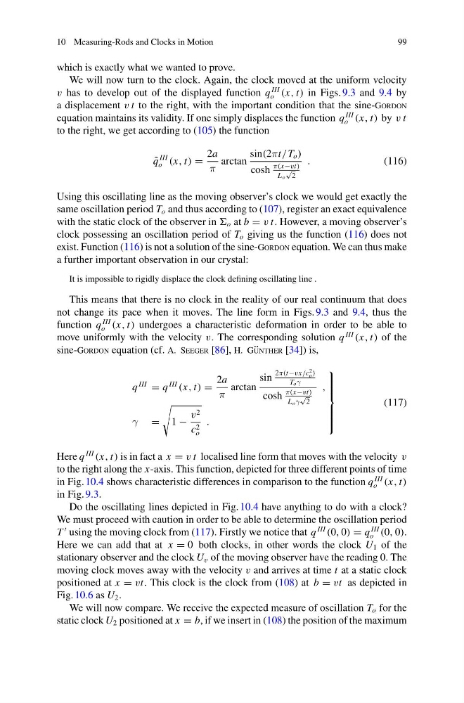
Using this oscillating line as the moving observer’s clock we would get exactly the
same oscillation period T o and thus according to (107), register an exact equivalence
with the static clock of the observer in o at b = v t. However, a moving observer’s
clock possessing an oscillation period of T o giving us the function (116) does not
exist. Function (116) is not a solution of the sine-Gordon equation. We can thus make
a further important observation in our crystal:
It is impossible to rigidly displace the clock defining oscillating line .
This means that there is no clock in the reality of our real continuum that does
not change its pace when it moves. The line form in Figs. 9.3 and 9.4, thus the
function q
III
o (x, t) undergoes a characteristic deformation in order to be able to
move uniformly with the velocity v. The corresponding solution q
III
(x, t) of the
sine-Gordon equation (cf. A. Seeger [86], H. G¨ unther [34]) is,
q
III
= q
III
(x, t) =
2a
π
arctan
sin
2π(t−vx/c
2
o )
T o γ
cosh
π(x−vt)
L o γ
√
2
,
γ =
1 −
v 2
c 2
o
.
⎫
⎪ ⎪ ⎪ ⎪ ⎬
⎪ ⎪ ⎪ ⎪ ⎭
(117)
Here q
III
(x, t) is in fact a x = v t localised line form that moves with the velocity v
to the right along the x-axis. This function, depicted for three different points of time
in Fig. 10.4 shows characteristic differences in comparison to the function q
III
o (x, t)
in Fig. 9.3.
Do the oscillating lines depicted in Fig. 10.4 have anything to do with a clock?
We must proceed with caution in order to be able to determine the oscillation period
T
using the moving clock from (117). Firstly we notice that q
III
(0, 0) = q
III
o (0, 0).
Here we can add that at x = 0 both clocks, in other words the clock U 1 of the
stationary observer and the clock U v of the moving observer have the reading 0. The
moving clock moves away with the velocity v and arrives at time t at a static clock
positioned at x = vt. This clock is the clock from (108) at b = vt as depicted in
Fig. 10.6 as U 2 .
We will now compare. We receive the expected measure of oscillation T o for the
static clock U 2 positioned at x = b, if we insert in (108) the position of the maximum
99
which is exactly what we wanted to prove.
We will now turn to the clock. Again, the clock moved at the uniform velocity
v has to develop out of the displayed function q
III
o (x, t) in Figs. 9.3 and 9.4 by
a displacement v t to the right, with the important condition that the sine-Gordon
equation maintains its validity. If one simply displaces the function q
III
o (x, t) by v t
to the right, we get according to (105) the function
˜
q
III
o (x, t) =
2a
π
arctan
sin(2πt/T o )
cosh
π(x−vt)
L o
√
2
.
(116)
Using this oscillating line as the moving observer’s clock we would get exactly the
same oscillation period T o and thus according to (107), register an exact equivalence
with the static clock of the observer in o at b = v t. However, a moving observer’s
clock possessing an oscillation period of T o giving us the function (116) does not
exist. Function (116) is not a solution of the sine-Gordon equation. We can thus make
a further important observation in our crystal:
It is impossible to rigidly displace the clock defining oscillating line .
This means that there is no clock in the reality of our real continuum that does
not change its pace when it moves. The line form in Figs. 9.3 and 9.4, thus the
function q
III
o (x, t) undergoes a characteristic deformation in order to be able to
move uniformly with the velocity v. The corresponding solution q
III
(x, t) of the
sine-Gordon equation (cf. A. Seeger [86], H. G¨ unther [34]) is,
q
III
= q
III
(x, t) =
2a
π
arctan
sin
2π(t−vx/c
2
o )
T o γ
cosh
π(x−vt)
L o γ
√
2
,
γ =
1 −
v 2
c 2
o
.
⎫
⎪ ⎪ ⎪ ⎪ ⎬
⎪ ⎪ ⎪ ⎪ ⎭
(117)
Here q
III
(x, t) is in fact a x = v t localised line form that moves with the velocity v
to the right along the x-axis. This function, depicted for three different points of time
in Fig. 10.4 shows characteristic differences in comparison to the function q
III
o (x, t)
in Fig. 9.3.
Do the oscillating lines depicted in Fig. 10.4 have anything to do with a clock?
We must proceed with caution in order to be able to determine the oscillation period
T
using the moving clock from (117). Firstly we notice that q
III
(0, 0) = q
III
o (0, 0).
Here we can add that at x = 0 both clocks, in other words the clock U 1 of the
stationary observer and the clock U v of the moving observer have the reading 0. The
moving clock moves away with the velocity v and arrives at time t at a static clock
positioned at x = vt. This clock is the clock from (108) at b = vt as depicted in
Fig. 10.6 as U 2 .
We will now compare. We receive the expected measure of oscillation T o for the
static clock U 2 positioned at x = b, if we insert in (108) the position of the maximum