

Solutions to exercises
45
As before, this relation can be simplified. For doped ThO 2 , when K e % K AF ,
we are led to consider a fourth range.
The diagram for the approximation becomes
n = 2[V
••
O ] D m = 2[V
••
O ]
p = D m
p = 2[O ′′
i ] log P O 2
Applying a reasoning identical to that of the previous question leads to
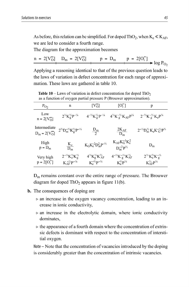
the laws of variation in defect concentration for each range of approximation. These laws are gathered in table 10.
Table 10 – Laws of variation in defect concentration for doped ThO 2
as a function of oxygen partial pressure P (Brouwer approximation).
P O 2
n
[V
••
O ]
[O′′ i ]
p
Low
n = 2[V
••
O ]
2
⅓
K
⅓
g P
−¹⁄6
4
−⅓
K
⅓
g P
−¹⁄6
4
⅓
K
−⅓
g K AF P
¹⁄6
2
−⅓
K
−⅓
g K e P
¹⁄6
Intermediate
D m = 2[V
••
O ]
2
½
D m
−½
K
½
g P
−¼
D
2
m
D
K
2
m
AF
2
−½
D m
½
K e K
−½
G P
¼
High
p = D m
D
K
m
e
K G K e
−2
D
2
m P
−½
K AF K G
−1
K e
2
D m
−2
P
½
D m
Very high
p = 2[O′′ i ]
2
−⅓
K
⅓
e K
⅓
g
K AF
−⅓
P
−¹⁄6
4
⅓
K
⅓
g K
⅔
AF
K e
−⅔
P
−¹⁄6
4
−⅓
K
−⅓
g K
⅓
AF
K e
⅔
P
¹⁄6
2
⅓
K e
⅔
K
−⅓
g
K
⅓
AF P
¹⁄6
D m remains constant over the entire range of pressure. The Brouwer
diagram for doped ThO 2 appears in figure 11(b).
b. The consequences of doping are
2 an increase in the oxygen vacancy concentration, leading to an increase in ionic conductivity,
2 an increase in the electrolytic domain, where ionic conductivity
dominates,
2 the appearance of a fourth domain where the concentration of extrinsic defects is dominant with respect to the concentration of interstitial oxygen.
Note – Note that the concentration of vacancies introduced by the doping
is considerably greater than the concentration of intrinsic vacancies.
45
As before, this relation can be simplified. For doped ThO 2 , when K e % K AF ,
we are led to consider a fourth range.
The diagram for the approximation becomes
n = 2[V
••
O ] D m = 2[V
••
O ]
p = D m
p = 2[O ′′
i ] log P O 2
Applying a reasoning identical to that of the previous question leads to
the laws of variation in defect concentration for each range of approximation. These laws are gathered in table 10.
Table 10 – Laws of variation in defect concentration for doped ThO 2
as a function of oxygen partial pressure P (Brouwer approximation).
P O 2
n
[V
••
O ]
[O′′ i ]
p
Low
n = 2[V
••
O ]
2
⅓
K
⅓
g P
−¹⁄6
4
−⅓
K
⅓
g P
−¹⁄6
4
⅓
K
−⅓
g K AF P
¹⁄6
2
−⅓
K
−⅓
g K e P
¹⁄6
Intermediate
D m = 2[V
••
O ]
2
½
D m
−½
K
½
g P
−¼
D
2
m
D
K
2
m
AF
2
−½
D m
½
K e K
−½
G P
¼
High
p = D m
D
K
m
e
K G K e
−2
D
2
m P
−½
K AF K G
−1
K e
2
D m
−2
P
½
D m
Very high
p = 2[O′′ i ]
2
−⅓
K
⅓
e K
⅓
g
K AF
−⅓
P
−¹⁄6
4
⅓
K
⅓
g K
⅔
AF
K e
−⅔
P
−¹⁄6
4
−⅓
K
−⅓
g K
⅓
AF
K e
⅔
P
¹⁄6
2
⅓
K e
⅔
K
−⅓
g
K
⅓
AF P
¹⁄6
D m remains constant over the entire range of pressure. The Brouwer
diagram for doped ThO 2 appears in figure 11(b).
b. The consequences of doping are
2 an increase in the oxygen vacancy concentration, leading to an increase in ionic conductivity,
2 an increase in the electrolytic domain, where ionic conductivity
dominates,
2 the appearance of a fourth domain where the concentration of extrinsic defects is dominant with respect to the concentration of interstitial oxygen.
Note – Note that the concentration of vacancies introduced by the doping
is considerably greater than the concentration of intrinsic vacancies.