

� �
�
�
55
2.5. Axial symmetry
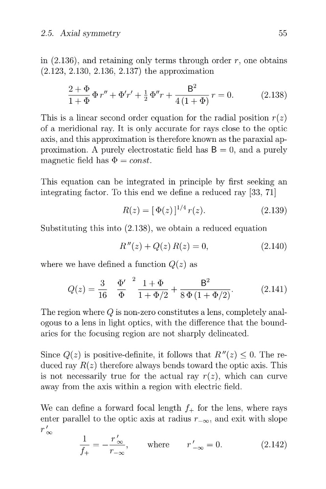
in (2.136), and retaining only terms through order r, one obtains
(2.123, 2.130, 2.136, 2.137) the approximation
B
2
2 + Φ
�
1 Φ
��
Φ r
�� + Φ
� r +
r +
r = 0.
(2.138)
1 + Φ
2
4 (1 + Φ)
This is a linear second order equation for the radial position r(z)
of a meridional ray. It is only accurate for rays close to the optic
axis, and this approximation is therefore known as the paraxial approximation. A purely electrostatic field has B = 0, and a purely
magnetic field has Φ = const.
This equation can be integrated in principle by first seeking an
integrating factor. To this end we define a reduced ray [33, 71]
R(z) = [ Φ(z) ]
1/4 r(z).
(2.139)
Substituting this into (2.138), we obtain a reduced equation
R
�� (z) + Q(z) R(z) = 0,
(2.140)
where we have defined a function Q(z) as
3 Φ
� 2 1 + Φ
B
2
Q(z) =
+
.
(2.141)
16 Φ
1 + Φ/2 8 Φ (1 + Φ/2)
The region where Q is non-zero constitutes a lens, completely analogous to a lens in light optics, with the difference that the boundaries for the focusing region are not sharply delineated.
Since Q(z) is positive-definite, it follows that R
�� (z) ≤ 0. The reduced ray R(z) therefore always bends toward the optic axis. This
is not necessarily true for the actual ray r(z), which can curve
away from the axis within a region with electric field.
We can define a forward focal length f + for the lens, where rays
enter parallel to the optic axis at radius r −∞ , and exit with slope
r ∞
1
r
= −
∞ ,
where
r −∞
�
= 0.
(2.142)
f +
r −∞
�
�
55
2.5. Axial symmetry
in (2.136), and retaining only terms through order r, one obtains
(2.123, 2.130, 2.136, 2.137) the approximation
B
2
2 + Φ
�
1 Φ
��
Φ r
�� + Φ
� r +
r +
r = 0.
(2.138)
1 + Φ
2
4 (1 + Φ)
This is a linear second order equation for the radial position r(z)
of a meridional ray. It is only accurate for rays close to the optic
axis, and this approximation is therefore known as the paraxial approximation. A purely electrostatic field has B = 0, and a purely
magnetic field has Φ = const.
This equation can be integrated in principle by first seeking an
integrating factor. To this end we define a reduced ray [33, 71]
R(z) = [ Φ(z) ]
1/4 r(z).
(2.139)
Substituting this into (2.138), we obtain a reduced equation
R
�� (z) + Q(z) R(z) = 0,
(2.140)
where we have defined a function Q(z) as
3 Φ
� 2 1 + Φ
B
2
Q(z) =
+
.
(2.141)
16 Φ
1 + Φ/2 8 Φ (1 + Φ/2)
The region where Q is non-zero constitutes a lens, completely analogous to a lens in light optics, with the difference that the boundaries for the focusing region are not sharply delineated.
Since Q(z) is positive-definite, it follows that R
�� (z) ≤ 0. The reduced ray R(z) therefore always bends toward the optic axis. This
is not necessarily true for the actual ray r(z), which can curve
away from the axis within a region with electric field.
We can define a forward focal length f + for the lens, where rays
enter parallel to the optic axis at radius r −∞ , and exit with slope
r ∞
1
r
= −
∞ ,
where
r −∞
�
= 0.
(2.142)
f +
r −∞