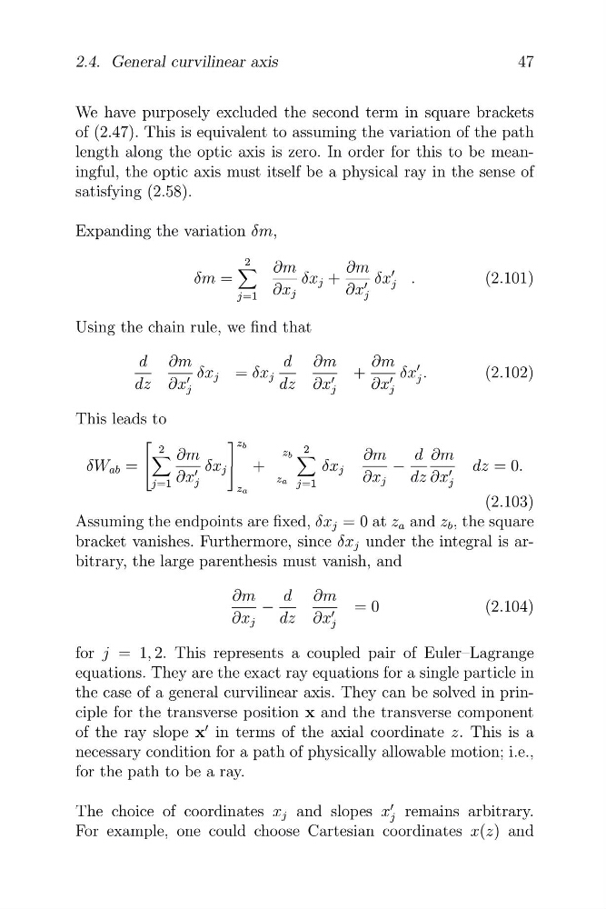
�
�
�
�
�
�
�
�
�
�
We have purposely excluded the second term in square brackets
of (2.47). This is equivalent to assuming the variation of the path
length along the optic axis is zero. In order for this to be meaningful, the optic axis must itself be a physical ray in the sense of
satisfying (2.58).
Expanding the variation δm,
2
4 ∂m
∂m
δm =
δx j +
δx j
�
.
(2.101)
∂x j
∂x
�
j=1
j
Using the chain rule, we find that
d ∂m
d ∂m
∂m
δx j = δx j
+
δx
�
j .
(2.102)
dz ∂x
�
dz ∂x
�
∂x
�
j
j
j
This leads to
⎡
⎤ z b
2
2
4
z b 4
∂m
∂m
d ∂m
δW ab = ⎣
δx j ⎦ +
δx j
−
dz = 0.
∂x
�
za
∂x j
dz ∂x
�
j=1
j
j=1
j
za
(2.103)
Assuming the endpoints are fixed, δx j = 0 at z a and z b , the square
bracket vanishes. Furthermore, since δx j under the integral is arbitrary, the large parenthesis must vanish, and
∂m
d ∂m
−
= 0
(2.104)
∂x j
dz ∂x j
�
for j = 1, 2. This represents a coupled pair of Euler–Lagrange
equations. They are the exact ray equations for a single particle in
the case of a general curvilinear axis. They can be solved in principle for the transverse position x and the transverse component
of the ray slope x
� in terms of the axial coordinate z. This is a
necessary condition for a path of physically allowable motion; i.e.,
for the path to be a ray.
The choice of coordinates x j and slopes x
�
j remains arbitrary.
For example, one could choose Cartesian coordinates x(z) and
47
2.4. General curvilinear axis