

45
2.4. General curvilinear axis
2.4 General curvilinear axis
For many systems, it is convenient to formulate the optics in terms
of transverse coordinates in a plane which is locally perpendicular
to a central optic axis. As this axis need not be a straight line,
we designate it a general curvilinear axis. We designate an axial
coordinate z, and transverse Cartesian coordinates x j = (x, y) for
j = (1, 2) in a plane locally perpendicular to the axis. We further
designate ray slope components x j
� = (x
� , y
� ) = dx j /dz. A ray is
completely specified at any plane z by its two-vector transverse
position x and its two-vector slope x
� .
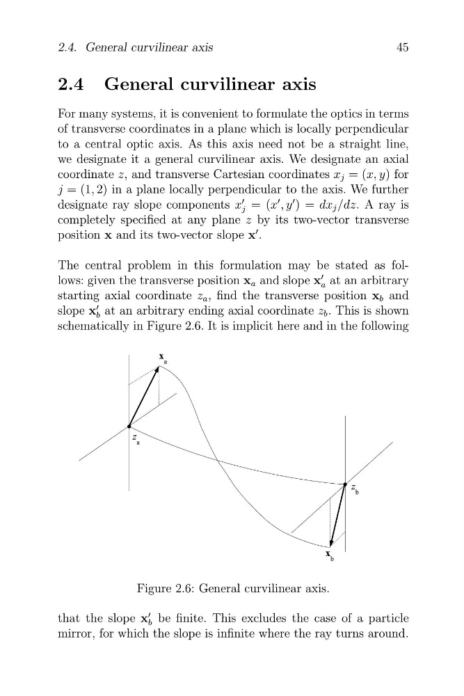
The central problem in this formulation may be stated as follows: given the transverse position x a and slope x
�
a at an arbitrary
starting axial coordinate z a , find the transverse position x b and
slope x
�
b at an arbitrary ending axial coordinate z b . This is shown
schematically in Figure 2.6. It is implicit here and in the following
Figure 2.6: General curvilinear axis.
that the slope x b
� be finite. This excludes the case of a particle
mirror, for which the slope is infinite where the ray turns around.
2.4. General curvilinear axis
2.4 General curvilinear axis
For many systems, it is convenient to formulate the optics in terms
of transverse coordinates in a plane which is locally perpendicular
to a central optic axis. As this axis need not be a straight line,
we designate it a general curvilinear axis. We designate an axial
coordinate z, and transverse Cartesian coordinates x j = (x, y) for
j = (1, 2) in a plane locally perpendicular to the axis. We further
designate ray slope components x j
� = (x
� , y
� ) = dx j /dz. A ray is
completely specified at any plane z by its two-vector transverse
position x and its two-vector slope x
� .
The central problem in this formulation may be stated as follows: given the transverse position x a and slope x
�
a at an arbitrary
starting axial coordinate z a , find the transverse position x b and
slope x
�
b at an arbitrary ending axial coordinate z b . This is shown
schematically in Figure 2.6. It is implicit here and in the following
Figure 2.6: General curvilinear axis.
that the slope x b
� be finite. This excludes the case of a particle
mirror, for which the slope is infinite where the ray turns around.