

22
Chapter 2. Geometrical optics
All relevant information about the magnetic and electric fields
is contained in the magnetic vector potential A(x, t) and electrostatic scalar potential φ(x, t), respectively. In general they are
functions of position x and time t, measured in the particular reference frame of interest. The potentials arise from source currents
and charges which are distributed in proximity to the charged particle of interest. They also include the effects of magnetic materials
and dielectrics. We assume in the following analysis that the potentials A(x, t) and φ(x, t) are known. The reader is referred to a
definitive text by Jackson [48], which describes how to calculate
these potentials, given a known distribution of charges, currents,
conductors, dielectrics, and magnetic materials.
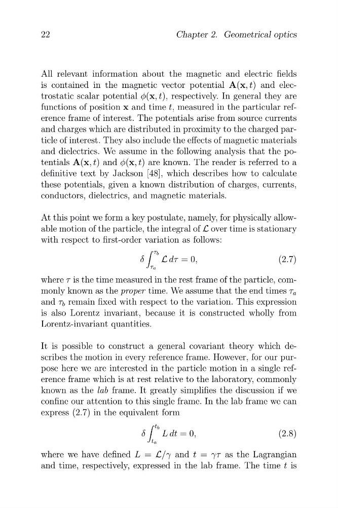
At this point we form a key postulate, namely, for physically allowable motion of the particle, the integral of L over time is stationary
with respect to first-order variation as follows:
τ b
δ
L dτ = 0,
(2.7)
τa
where τ is the time measured in the rest frame of the particle, commonly known as the proper time. We assume that the end times τ a
and τ b remain fixed with respect to the variation. This expression
is also Lorentz invariant, because it is constructed wholly from
Lorentz-invariant quantities.
It is possible to construct a general covariant theory which describes the motion in every reference frame. However, for our purpose here we are interested in the particle motion in a single reference frame which is at rest relative to the laboratory, commonly
known as the lab frame. It greatly simplifies the discussion if we
confine our attention to this single frame. In the lab frame we can
express (2.7) in the equivalent form
t b
δ
L dt = 0,
(2.8)
ta
where we have defined L = L/γ and t = γτ as the Lagrangian
and time, respectively, expressed in the lab frame. The time t is
Chapter 2. Geometrical optics
All relevant information about the magnetic and electric fields
is contained in the magnetic vector potential A(x, t) and electrostatic scalar potential φ(x, t), respectively. In general they are
functions of position x and time t, measured in the particular reference frame of interest. The potentials arise from source currents
and charges which are distributed in proximity to the charged particle of interest. They also include the effects of magnetic materials
and dielectrics. We assume in the following analysis that the potentials A(x, t) and φ(x, t) are known. The reader is referred to a
definitive text by Jackson [48], which describes how to calculate
these potentials, given a known distribution of charges, currents,
conductors, dielectrics, and magnetic materials.
At this point we form a key postulate, namely, for physically allowable motion of the particle, the integral of L over time is stationary
with respect to first-order variation as follows:
τ b
δ
L dτ = 0,
(2.7)
τa
where τ is the time measured in the rest frame of the particle, commonly known as the proper time. We assume that the end times τ a
and τ b remain fixed with respect to the variation. This expression
is also Lorentz invariant, because it is constructed wholly from
Lorentz-invariant quantities.
It is possible to construct a general covariant theory which describes the motion in every reference frame. However, for our purpose here we are interested in the particle motion in a single reference frame which is at rest relative to the laboratory, commonly
known as the lab frame. It greatly simplifies the discussion if we
confine our attention to this single frame. In the lab frame we can
express (2.7) in the equivalent form
t b
δ
L dt = 0,
(2.8)
ta
where we have defined L = L/γ and t = γτ as the Lagrangian
and time, respectively, expressed in the lab frame. The time t is