

�
�
311
5.4. Field emission
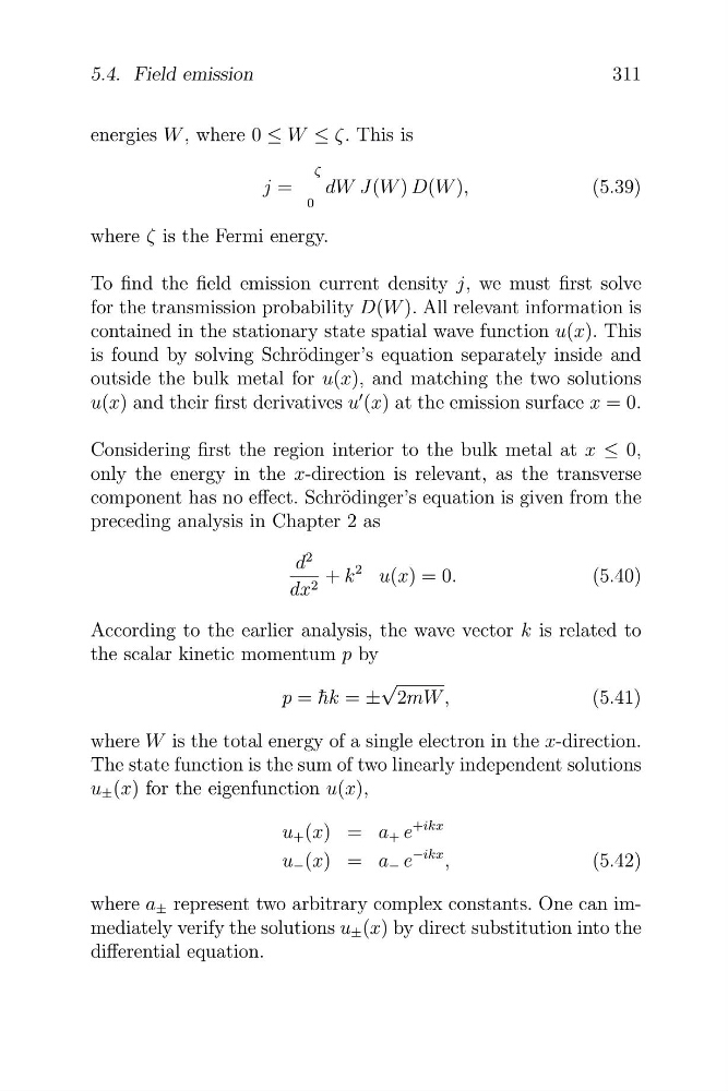
energies W , where 0 ≤ W ≤ ζ. This is
ζ
j =
dW J(W ) D(W ),
(5.39)
0
where ζ is the Fermi energy.
To find the field emission current density j, we must first solve
for the transmission probability D(W ). All relevant information is
contained in the stationary state spatial wave function u(x). This
is found by solving Schr¨ odinger’s equation separately inside and
outside the bulk metal for u(x), and matching the two solutions
u(x) and their first derivatives u
� (x) at the emission surface x = 0.
Considering first the region interior to the bulk metal at x ≤ 0,
only the energy in the x-direction is relevant, as the transverse
component has no effect. Schr¨ odinger’s equation is given from the
preceding analysis in Chapter 2 as
d
2
+ k
2 u(x) = 0.
(5.40)
dx 2
According to the earlier analysis, the wave vector k is related to
the scalar kinetic momentum p by
√
p = ¯
hk = ± 2mW ,
(5.41)
where W is the total energy of a single electron in the x-direction.
The state function is the sum of two linearly independent solutions
u ± (x) for the eigenfunction u(x),
=
+ikx
u + (x)
a + e
u − (x) = a − e
−ikx ,
(5.42)
where a ± represent two arbitrary complex constants. One can immediately verify the solutions u ± (x) by direct substitution into the
differential equation.
�
311
5.4. Field emission
energies W , where 0 ≤ W ≤ ζ. This is
ζ
j =
dW J(W ) D(W ),
(5.39)
0
where ζ is the Fermi energy.
To find the field emission current density j, we must first solve
for the transmission probability D(W ). All relevant information is
contained in the stationary state spatial wave function u(x). This
is found by solving Schr¨ odinger’s equation separately inside and
outside the bulk metal for u(x), and matching the two solutions
u(x) and their first derivatives u
� (x) at the emission surface x = 0.
Considering first the region interior to the bulk metal at x ≤ 0,
only the energy in the x-direction is relevant, as the transverse
component has no effect. Schr¨ odinger’s equation is given from the
preceding analysis in Chapter 2 as
d
2
+ k
2 u(x) = 0.
(5.40)
dx 2
According to the earlier analysis, the wave vector k is related to
the scalar kinetic momentum p by
√
p = ¯
hk = ± 2mW ,
(5.41)
where W is the total energy of a single electron in the x-direction.
The state function is the sum of two linearly independent solutions
u ± (x) for the eigenfunction u(x),
=
+ikx
u + (x)
a + e
u − (x) = a − e
−ikx ,
(5.42)
where a ± represent two arbitrary complex constants. One can immediately verify the solutions u ± (x) by direct substitution into the
differential equation.