

3.2. Particle motion in a general electromagnetic potential 161
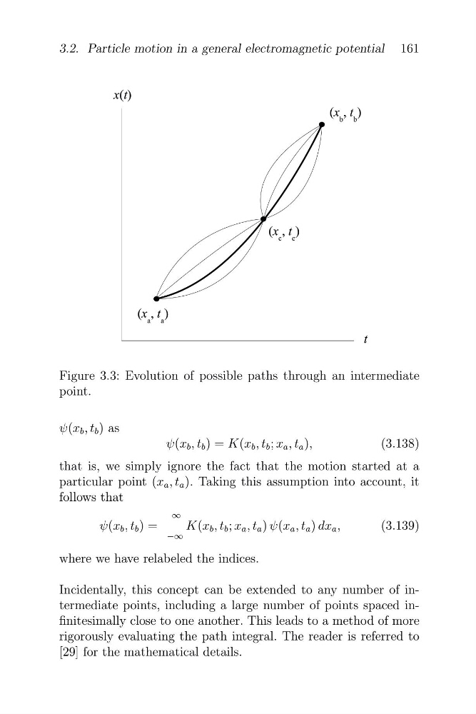
Figure 3.3: Evolution of possible paths through an intermediate
point.
ψ(x b , t b ) as
ψ(x b , t b ) = K(x b , t b ; x a , t a ),
(3.138)
that is, we simply ignore the fact that the motion started at a
particular point (x a , t a ). Taking this assumption into account, it
follows that
∞
ψ(x b , t b ) =
K(x b , t b ; x a , t a ) ψ(x a , t a ) dx a ,
(3.139)
−∞
where we have relabeled the indices.
Incidentally, this concept can be extended to any number of intermediate points, including a large number of points spaced infinitesimally close to one another. This leads to a method of more
rigorously evaluating the path integral. The reader is referred to
[29] for the mathematical details.
Figure 3.3: Evolution of possible paths through an intermediate
point.
ψ(x b , t b ) as
ψ(x b , t b ) = K(x b , t b ; x a , t a ),
(3.138)
that is, we simply ignore the fact that the motion started at a
particular point (x a , t a ). Taking this assumption into account, it
follows that
∞
ψ(x b , t b ) =
K(x b , t b ; x a , t a ) ψ(x a , t a ) dx a ,
(3.139)
−∞
where we have relabeled the indices.
Incidentally, this concept can be extended to any number of intermediate points, including a large number of points spaced infinitesimally close to one another. This leads to a method of more
rigorously evaluating the path integral. The reader is referred to
[29] for the mathematical details.