

THz Bandpass Filter Design Using Metamaterial-Based Defected 1D …
7
and for TM polarization
n left →
cos θ left
n left
n right →
cos θ right
n right
(3.22)
3.2 Eigenmodes for Planar Photonic Structure
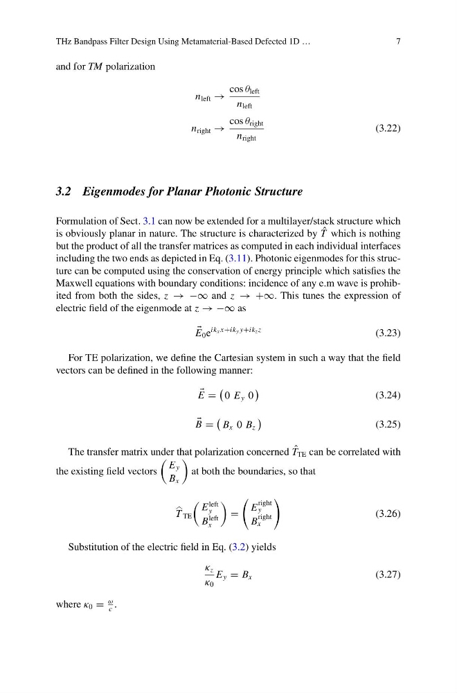
Formulation of Sect. 3.1 can now be extended for a multilayer/stack structure which
is obviously planar in nature. The structure is characterized by ˆ
T which is nothing
but the product of all the transfer matrices as computed in each individual interfaces
including the two ends as depicted in Eq. (3.11). Photonic eigenmodes for this structure can be computed using the conservation of energy principle which satisfies the
Maxwell equations with boundary conditions: incidence of any e.m wave is prohibited from both the sides, z → −∞ and z → +∞. This tunes the expression of
electric field of the eigenmode at z → −∞ as
E 0 e
ik x x+ik y y+ik z z
(3.23)
For TE polarization, we define the Cartesian system in such a way that the field
vectors can be defined in the following manner:
E =
0 E y 0
(3.24)
B =
B x 0 B z
(3.25)
The transfer matrix under that polarization concerned ˆ
T TE can be correlated with
the existing field vectors
E y
B x
at both the boundaries, so that
T
TE
E
left
y
B
left
x
=
E
right
y
B
right
x
(3.26)
Substitution of the electric field in Eq. (3.2) yields
κ z
κ 0
E y = B x
(3.27)
where κ 0 =
ω
c
.
7
and for TM polarization
n left →
cos θ left
n left
n right →
cos θ right
n right
(3.22)
3.2 Eigenmodes for Planar Photonic Structure
Formulation of Sect. 3.1 can now be extended for a multilayer/stack structure which
is obviously planar in nature. The structure is characterized by ˆ
T which is nothing
but the product of all the transfer matrices as computed in each individual interfaces
including the two ends as depicted in Eq. (3.11). Photonic eigenmodes for this structure can be computed using the conservation of energy principle which satisfies the
Maxwell equations with boundary conditions: incidence of any e.m wave is prohibited from both the sides, z → −∞ and z → +∞. This tunes the expression of
electric field of the eigenmode at z → −∞ as
E 0 e
ik x x+ik y y+ik z z
(3.23)
For TE polarization, we define the Cartesian system in such a way that the field
vectors can be defined in the following manner:
E =
0 E y 0
(3.24)
B =
B x 0 B z
(3.25)
The transfer matrix under that polarization concerned ˆ
T TE can be correlated with
the existing field vectors
E y
B x
at both the boundaries, so that
T
TE
E
left
y
B
left
x
=
E
right
y
B
right
x
(3.26)
Substitution of the electric field in Eq. (3.2) yields
κ z
κ 0
E y = B x
(3.27)
where κ 0 =
ω
c
.