

88
R. S. Stankovi´ c et al.
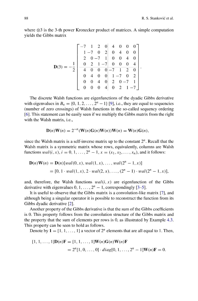
where ⊗3 is the 3-th power Kronecker product of matrices. A simple computation
yields the Gibbs matrix
D(3) = −
1
2
⎡
⎢
⎢
⎢
⎢
⎢
⎢
⎢
⎢
⎢
⎢
⎢
⎣
−7 1 2 0 4 0 0 0
1 −7 0 2 0 4 0 0
2 0 −7 1 0 0 4 0
0 2 1 −7 0 0 0 4
4 0 0 0 −7 1 2 0
0 4 0 0 1 −7 0 2
0 0 4 0 2 0 −7 1
0 0 0 4 0 2 1 −7
⎤
⎥
⎥
⎥
⎥
⎥
⎥
⎥
⎥
⎥
⎥
⎥
⎦
.
The discrete Walsh functions are eigenfunctions of the dyadic Gibbs derivative
with eigenvalues in B n = {0, 1, 2, . . . , 2 n − 1} [9], i.e., they are equal to sequencies
(number of zero crossings) of Walsh functions in the so-called sequency ordering
[6]. This statement can be easily seen if we multiply the Gibbs matrix from the right
with the Walsh matrix, i.e.,
D(n)W(n) = 2
−n (W(n)G(n)W(n))W(n) = W(n)G(n),
since the Walsh matrix is a self-inverse matrix up to the constant 2 n . Recall that the
Walsh matrix is a symmetric matrix whose rows, equivalently, columns are Walsh
functions wal(i, x), i = 0, 1, . . . , 2 n − 1, x = (x 1 , x 2 , . . . , x n ), and it follows:
D(n)W(n) = D(n)[wal(0, x), wal(1, x), . . . , wal(2
n
− 1, x)]
= [0, 1 · wal(1, x), 2 · wal(2, x), . . . , (2
n
− 1) · wal(2
n
− 1, x)],
and, therefore, the Walsh functions wal(i, x) are eigenfunction of the Gibbs
derivative with eigenvalues 0, 1, . . . , 2 n − 1, correspondingly [3–5].
It is useful to observe that the Gibbs matrix is a convolution-like matrix [7], and
although being a singular operator it is possible to reconstruct the function from its
Gibbs dyadic derivative [2].
Another property of the Gibbs derivative is that the sum of the Gibbs coefficients
is 0. This property follows from the convolution structure of the Gibbs matrix and
the property that the sum of elements per rows is 0, as illustrated by Example 4.3.
This property can be seen to hold as follows.
Denote by 1 = [1, 1, . . . , 1] a vector of 2 n elements that are all equal to 1. Then,
[1, 1, . . . , 1]D(n)F = [1, 1, . . . , 1]W(n)G(n)W(n)F
= 2
n
[1, 0, . . . , 0] · diag[0, 1, . . . , 2
n
− 1]W(n)F = 0.
R. S. Stankovi´ c et al.
where ⊗3 is the 3-th power Kronecker product of matrices. A simple computation
yields the Gibbs matrix
D(3) = −
1
2
⎡
⎢
⎢
⎢
⎢
⎢
⎢
⎢
⎢
⎢
⎢
⎢
⎣
−7 1 2 0 4 0 0 0
1 −7 0 2 0 4 0 0
2 0 −7 1 0 0 4 0
0 2 1 −7 0 0 0 4
4 0 0 0 −7 1 2 0
0 4 0 0 1 −7 0 2
0 0 4 0 2 0 −7 1
0 0 0 4 0 2 1 −7
⎤
⎥
⎥
⎥
⎥
⎥
⎥
⎥
⎥
⎥
⎥
⎥
⎦
.
The discrete Walsh functions are eigenfunctions of the dyadic Gibbs derivative
with eigenvalues in B n = {0, 1, 2, . . . , 2 n − 1} [9], i.e., they are equal to sequencies
(number of zero crossings) of Walsh functions in the so-called sequency ordering
[6]. This statement can be easily seen if we multiply the Gibbs matrix from the right
with the Walsh matrix, i.e.,
D(n)W(n) = 2
−n (W(n)G(n)W(n))W(n) = W(n)G(n),
since the Walsh matrix is a self-inverse matrix up to the constant 2 n . Recall that the
Walsh matrix is a symmetric matrix whose rows, equivalently, columns are Walsh
functions wal(i, x), i = 0, 1, . . . , 2 n − 1, x = (x 1 , x 2 , . . . , x n ), and it follows:
D(n)W(n) = D(n)[wal(0, x), wal(1, x), . . . , wal(2
n
− 1, x)]
= [0, 1 · wal(1, x), 2 · wal(2, x), . . . , (2
n
− 1) · wal(2
n
− 1, x)],
and, therefore, the Walsh functions wal(i, x) are eigenfunction of the Gibbs
derivative with eigenvalues 0, 1, . . . , 2 n − 1, correspondingly [3–5].
It is useful to observe that the Gibbs matrix is a convolution-like matrix [7], and
although being a singular operator it is possible to reconstruct the function from its
Gibbs dyadic derivative [2].
Another property of the Gibbs derivative is that the sum of the Gibbs coefficients
is 0. This property follows from the convolution structure of the Gibbs matrix and
the property that the sum of elements per rows is 0, as illustrated by Example 4.3.
This property can be seen to hold as follows.
Denote by 1 = [1, 1, . . . , 1] a vector of 2 n elements that are all equal to 1. Then,
[1, 1, . . . , 1]D(n)F = [1, 1, . . . , 1]W(n)G(n)W(n)F
= 2
n
[1, 0, . . . , 0] · diag[0, 1, . . . , 2
n
− 1]W(n)F = 0.