

208
D. M. Miller and M. Soeken
0
500
1000
1500
2000
2500
3000
1
6
11 16 21 26 31 36 41 46 51 56 61 66 71 76 81 86 91
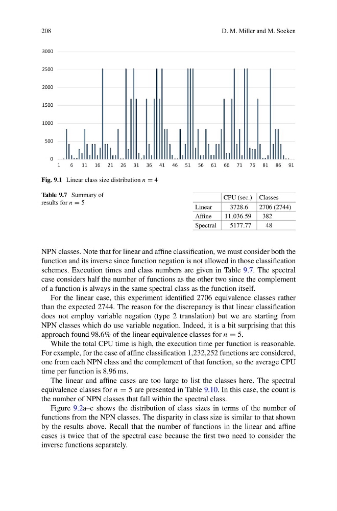
Fig. 9.1 Linear class size distribution n = 4
Table 9.7 Summary of
results for n = 5
CPU (sec.) Classes
Linear
3728.6
2706 (2744)
Affine
11,036.59
382
Spectral
5177.77
48
NPN classes. Note that for linear and affine classification, we must consider both the
function and its inverse since function negation is not allowed in those classification
schemes. Execution times and class numbers are given in Table 9.7. The spectral
case considers half the number of functions as the other two since the complement
of a function is always in the same spectral class as the function itself.
For the linear case, this experiment identified 2706 equivalence classes rather
than the expected 2744. The reason for the discrepancy is that linear classification
does not employ variable negation (type 2 translation) but we are starting from
NPN classes which do use variable negation. Indeed, it is a bit surprising that this
approach found 98.6% of the linear equivalence classes for n = 5.
While the total CPU time is high, the execution time per function is reasonable.
For example, for the case of affine classification 1,232,252 functions are considered,
one from each NPN class and the complement of that function, so the average CPU
time per function is 8.96 ms.
The linear and affine cases are too large to list the classes here. The spectral
equivalence classes for n = 5 are presented in Table 9.10. In this case, the count is
the number of NPN classes that fall within the spectral class.
Figure 9.2a–c shows the distribution of class sizes in terms of the number of
functions from the NPN classes. The disparity in class size is similar to that shown
by the results above. Recall that the number of functions in the linear and affine
cases is twice that of the spectral case because the first two need to consider the
inverse functions separately.
D. M. Miller and M. Soeken
0
500
1000
1500
2000
2500
3000
1
6
11 16 21 26 31 36 41 46 51 56 61 66 71 76 81 86 91
Fig. 9.1 Linear class size distribution n = 4
Table 9.7 Summary of
results for n = 5
CPU (sec.) Classes
Linear
3728.6
2706 (2744)
Affine
11,036.59
382
Spectral
5177.77
48
NPN classes. Note that for linear and affine classification, we must consider both the
function and its inverse since function negation is not allowed in those classification
schemes. Execution times and class numbers are given in Table 9.7. The spectral
case considers half the number of functions as the other two since the complement
of a function is always in the same spectral class as the function itself.
For the linear case, this experiment identified 2706 equivalence classes rather
than the expected 2744. The reason for the discrepancy is that linear classification
does not employ variable negation (type 2 translation) but we are starting from
NPN classes which do use variable negation. Indeed, it is a bit surprising that this
approach found 98.6% of the linear equivalence classes for n = 5.
While the total CPU time is high, the execution time per function is reasonable.
For example, for the case of affine classification 1,232,252 functions are considered,
one from each NPN class and the complement of that function, so the average CPU
time per function is 8.96 ms.
The linear and affine cases are too large to list the classes here. The spectral
equivalence classes for n = 5 are presented in Table 9.10. In this case, the count is
the number of NPN classes that fall within the spectral class.
Figure 9.2a–c shows the distribution of class sizes in terms of the number of
functions from the NPN classes. The disparity in class size is similar to that shown
by the results above. Recall that the number of functions in the linear and affine
cases is twice that of the spectral case because the first two need to consider the
inverse functions separately.