

6 Synthesis of Majority Expressions Through Primitive Function Manipulation
139
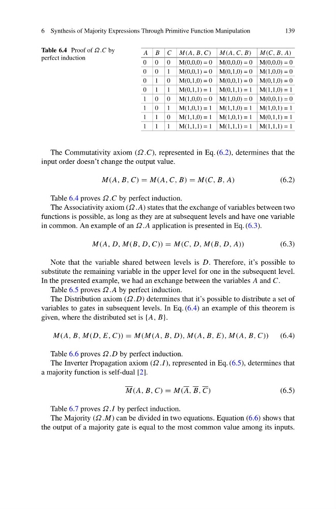
Table 6.4 Proof of Ω.C by
perfect induction
A B C M(A, B, C) M(A, C, B) M(C, B, A)
0 0 0 M(0,0,0) = 0 M(0,0,0) = 0 M(0,0,0) = 0
0 0 1 M(0,0,1) = 0 M(0,1,0) = 0 M(1,0,0) = 0
0 1 0 M(0,1,0) = 0 M(0,0,1) = 0 M(0,1,0) = 0
0 1 1 M(0,1,1) = 1 M(0,1,1) = 1 M(1,1,0) = 1
1 0 0 M(1,0,0) = 0 M(1,0,0) = 0 M(0,0,1) = 0
1 0 1 M(1,0,1) = 1 M(1,1,0) = 1 M(1,0,1) = 1
1 1 0 M(1,1,0) = 1 M(1,0,1) = 1 M(0,1,1) = 1
1 1 1 M(1,1,1) = 1 M(1,1,1) = 1 M(1,1,1) = 1
The Commutativity axiom (Ω.C), represented in Eq. (6.2), determines that the
input order doesn’t change the output value.
M(A, B, C) = M(A, C, B) = M(C, B, A)
(6.2)
Table 6.4 proves Ω.C by perfect induction.
The Associativity axiom (Ω.A) states that the exchange of variables between two
functions is possible, as long as they are at subsequent levels and have one variable
in common. An example of an Ω.A application is presented in Eq. (6.3).
M(A, D, M(B, D, C)) = M(C, D, M(B, D, A))
(6.3)
Note that the variable shared between levels is D. Therefore, it’s possible to
substitute the remaining variable in the upper level for one in the subsequent level.
In the presented example, we had an exchange between the variables A and C.
Table 6.5 proves Ω.A by perfect induction.
The Distribution axiom (Ω.D) determines that it’s possible to distribute a set of
variables to gates in subsequent levels. In Eq. (6.4) an example of this theorem is
given, where the distributed set is {A, B}.
M(A, B, M(D, E, C)) = M(M(A, B, D), M(A, B, E), M(A, B, C)) (6.4)
Table 6.6 proves Ω.D by perfect induction.
The Inverter Propagation axiom (Ω.I ), represented in Eq. (6.5), determines that
a majority function is self-dual [2].
M(A, B, C) = M(A, B, C)
(6.5)
Table 6.7 proves Ω.I by perfect induction.
The Majority (Ω.M) can be divided in two equations. Equation (6.6) shows that
the output of a majority gate is equal to the most common value among its inputs.
139
Table 6.4 Proof of Ω.C by
perfect induction
A B C M(A, B, C) M(A, C, B) M(C, B, A)
0 0 0 M(0,0,0) = 0 M(0,0,0) = 0 M(0,0,0) = 0
0 0 1 M(0,0,1) = 0 M(0,1,0) = 0 M(1,0,0) = 0
0 1 0 M(0,1,0) = 0 M(0,0,1) = 0 M(0,1,0) = 0
0 1 1 M(0,1,1) = 1 M(0,1,1) = 1 M(1,1,0) = 1
1 0 0 M(1,0,0) = 0 M(1,0,0) = 0 M(0,0,1) = 0
1 0 1 M(1,0,1) = 1 M(1,1,0) = 1 M(1,0,1) = 1
1 1 0 M(1,1,0) = 1 M(1,0,1) = 1 M(0,1,1) = 1
1 1 1 M(1,1,1) = 1 M(1,1,1) = 1 M(1,1,1) = 1
The Commutativity axiom (Ω.C), represented in Eq. (6.2), determines that the
input order doesn’t change the output value.
M(A, B, C) = M(A, C, B) = M(C, B, A)
(6.2)
Table 6.4 proves Ω.C by perfect induction.
The Associativity axiom (Ω.A) states that the exchange of variables between two
functions is possible, as long as they are at subsequent levels and have one variable
in common. An example of an Ω.A application is presented in Eq. (6.3).
M(A, D, M(B, D, C)) = M(C, D, M(B, D, A))
(6.3)
Note that the variable shared between levels is D. Therefore, it’s possible to
substitute the remaining variable in the upper level for one in the subsequent level.
In the presented example, we had an exchange between the variables A and C.
Table 6.5 proves Ω.A by perfect induction.
The Distribution axiom (Ω.D) determines that it’s possible to distribute a set of
variables to gates in subsequent levels. In Eq. (6.4) an example of this theorem is
given, where the distributed set is {A, B}.
M(A, B, M(D, E, C)) = M(M(A, B, D), M(A, B, E), M(A, B, C)) (6.4)
Table 6.6 proves Ω.D by perfect induction.
The Inverter Propagation axiom (Ω.I ), represented in Eq. (6.5), determines that
a majority function is self-dual [2].
M(A, B, C) = M(A, B, C)
(6.5)
Table 6.7 proves Ω.I by perfect induction.
The Majority (Ω.M) can be divided in two equations. Equation (6.6) shows that
the output of a majority gate is equal to the most common value among its inputs.