

5 Improving SAT Solving Using Monte Carlo Tree Search-Based Clause Learning
115
root
n
. . .
n p
. . .
. . .
. . .
n.counter = n.counter − n p .counter
n.value = n.value − n p .value
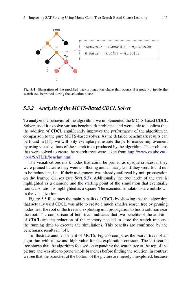
Fig. 5.4 Illustration of the modified backpropagation phase that occurs if a node n p inside the
search tree is pruned during the selection phase
5.3.2 Analysis of the MCTS-Based CDCL Solver
To analyze the behavior of the algorithm, we implemented the MCTS-based CDCL
Solver, used it to solve various benchmark problems, and were able to confirm that
the addition of CDCL significantly improves the performance of the algorithm in
comparison to the pure MCTS-based solver. As the detailed benchmark results can
be found in [14], we will only exemplary illustrate the performance improvement
by using visualizations of the search trees produced by the algorithm. The problems
that were solved to create the search trees were taken from http://www.cs.ubc.ca/~
hoos/SATLIB/benchm.html.
The visualizations mark nodes that could be pruned as opaque crosses, if they
were pruned because they were conflicting and as triangles, if they were found out
to be redundant, i.e., if their assignment was already enforced by unit propagation
on the learned clauses (see Sect. 5.3). Additionally the root node of the tree is
highlighted as a diamond and the starting point of the simulation that eventually
found a solution is highlighted as a square. The executed simulations are not shown
in the visualization.
Figure 5.5 illustrates the main benefits of CDCL by showing that the algorithm
that actually used CDCL was able to create a much smaller search tree by pruning
nodes near the root of the tree and exploiting unit propagation to find a solution near
the root. The comparison of both trees indicates that two benefits of the addition
of CDCL are the reduction of the memory needed to store the search tree and
the running time to execute the simulations. This benefits are confirmed by the
benchmark results in [14].
To illustrate another benefit of MCTS, Fig. 5.6 compares the search trees of an
algorithm with a low and high value for the exploration constant. The left search
tree shows that the algorithm focused on expanding the search tree at the top of the
picture and was able to prune whole branches before finding the solution. In contrast
we see that the branches at the bottom of the picture are merely unexplored, because
115
root
n
. . .
n p
. . .
. . .
. . .
n.counter = n.counter − n p .counter
n.value = n.value − n p .value
Fig. 5.4 Illustration of the modified backpropagation phase that occurs if a node n p inside the
search tree is pruned during the selection phase
5.3.2 Analysis of the MCTS-Based CDCL Solver
To analyze the behavior of the algorithm, we implemented the MCTS-based CDCL
Solver, used it to solve various benchmark problems, and were able to confirm that
the addition of CDCL significantly improves the performance of the algorithm in
comparison to the pure MCTS-based solver. As the detailed benchmark results can
be found in [14], we will only exemplary illustrate the performance improvement
by using visualizations of the search trees produced by the algorithm. The problems
that were solved to create the search trees were taken from http://www.cs.ubc.ca/~
hoos/SATLIB/benchm.html.
The visualizations mark nodes that could be pruned as opaque crosses, if they
were pruned because they were conflicting and as triangles, if they were found out
to be redundant, i.e., if their assignment was already enforced by unit propagation
on the learned clauses (see Sect. 5.3). Additionally the root node of the tree is
highlighted as a diamond and the starting point of the simulation that eventually
found a solution is highlighted as a square. The executed simulations are not shown
in the visualization.
Figure 5.5 illustrates the main benefits of CDCL by showing that the algorithm
that actually used CDCL was able to create a much smaller search tree by pruning
nodes near the root of the tree and exploiting unit propagation to find a solution near
the root. The comparison of both trees indicates that two benefits of the addition
of CDCL are the reduction of the memory needed to store the search tree and
the running time to execute the simulations. This benefits are confirmed by the
benchmark results in [14].
To illustrate another benefit of MCTS, Fig. 5.6 compares the search trees of an
algorithm with a low and high value for the exploration constant. The left search
tree shows that the algorithm focused on expanding the search tree at the top of the
picture and was able to prune whole branches before finding the solution. In contrast
we see that the branches at the bottom of the picture are merely unexplored, because