

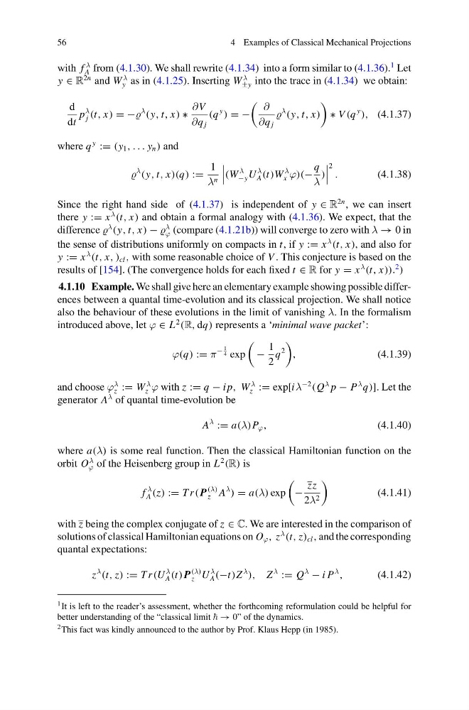
56
4 Examples of Classical Mechanical Projections
with f
λ
A from (4.1.30). We shall rewrite (4.1.34) into a form similar to (4.1.36).
1 Let
y ∈ R
2n and W
λ
y as in (4.1.25). Inserting W
λ
±y into the trace in (4.1.34) we obtain:
d
dt
p
λ
j (t, x) = −
λ
(y, t, x) ∗
∂V
∂q j
(q
y
) = −
∂
∂q j
λ
(y, t, x)
∗ V (q
y
), (4.1.37)
where q
y
:= (y 1 , . . . y n ) and
λ
(y, t, x)(q) :=
1
λ n
(W
λ
−y U
λ
A (t)W
λ
x ϕ)(−
q
λ
)
2 .
(4.1.38)
Since the right hand side of (4.1.37) is independent of y ∈ R
2n , we can insert
there y := x
λ
(t, x) and obtain a formal analogy with (4.1.36). We expect, that the
difference
λ
(y, t, x) −
λ
ϕ (compare (4.1.21b)) will converge to zero with λ → 0 in
the sense of distributions uniformly on compacts in t, if y := x
λ
(t, x), and also for
y := x
λ
(t, x, ) cl , with some reasonable choice of V . This conjecture is based on the
results of [154]. (The convergence holds for each fixed t ∈ R for y = x
λ
(t, x)).
2 )
4.1.10 Example. We shall give here an elementary example showing possible differences between a quantal time-evolution and its classical projection. We shall notice
also the behaviour of these evolutions in the limit of vanishing λ. In the formalism
introduced above, let ϕ ∈ L
2
(R, dq) represents a ‘minimal wave packet’:
ϕ(q) := π
−
1
4 exp
−
1
2
q
2
,
(4.1.39)
and choose ϕ
λ
z := W
λ
z ϕ with z := q − i p, W
λ
z := exp[iλ
−2
(Q
λ p − P
λ q)]. Let the
generator A
λ of quantal time-evolution be
A
λ
:= a(λ)P ϕ ,
(4.1.40)
where a(λ) is some real function. Then the classical Hamiltonian function on the
orbit O
λ
ϕ of the Heisenberg group in L
2
(R) is
f
λ
A (z) := T r( P
(λ)
z A
λ
) = a(λ) exp
−
zz
2λ 2
(4.1.41)
with z being the complex conjugate of z ∈ C. We are interested in the comparison of
solutions of classical Hamiltonian equations on O ϕ , z
λ
(t, z) cl , and the corresponding
quantal expectations:
z
λ
(t, z) := T r(U
λ
A (t) P
(λ)
z U
λ
A (−t)Z
λ
), Z
λ
:= Q
λ
− i P
λ
,
(4.1.42)
1 It is left to the reader’s assessment, whether the forthcoming reformulation could be helpful for
better understanding of the “classical limit → 0” of the dynamics.
2 This fact was kindly announced to the author by Prof. Klaus Hepp (in 1985).
4 Examples of Classical Mechanical Projections
with f
λ
A from (4.1.30). We shall rewrite (4.1.34) into a form similar to (4.1.36).
1 Let
y ∈ R
2n and W
λ
y as in (4.1.25). Inserting W
λ
±y into the trace in (4.1.34) we obtain:
d
dt
p
λ
j (t, x) = −
λ
(y, t, x) ∗
∂V
∂q j
(q
y
) = −
∂
∂q j
λ
(y, t, x)
∗ V (q
y
), (4.1.37)
where q
y
:= (y 1 , . . . y n ) and
λ
(y, t, x)(q) :=
1
λ n
(W
λ
−y U
λ
A (t)W
λ
x ϕ)(−
q
λ
)
2 .
(4.1.38)
Since the right hand side of (4.1.37) is independent of y ∈ R
2n , we can insert
there y := x
λ
(t, x) and obtain a formal analogy with (4.1.36). We expect, that the
difference
λ
(y, t, x) −
λ
ϕ (compare (4.1.21b)) will converge to zero with λ → 0 in
the sense of distributions uniformly on compacts in t, if y := x
λ
(t, x), and also for
y := x
λ
(t, x, ) cl , with some reasonable choice of V . This conjecture is based on the
results of [154]. (The convergence holds for each fixed t ∈ R for y = x
λ
(t, x)).
2 )
4.1.10 Example. We shall give here an elementary example showing possible differences between a quantal time-evolution and its classical projection. We shall notice
also the behaviour of these evolutions in the limit of vanishing λ. In the formalism
introduced above, let ϕ ∈ L
2
(R, dq) represents a ‘minimal wave packet’:
ϕ(q) := π
−
1
4 exp
−
1
2
q
2
,
(4.1.39)
and choose ϕ
λ
z := W
λ
z ϕ with z := q − i p, W
λ
z := exp[iλ
−2
(Q
λ p − P
λ q)]. Let the
generator A
λ of quantal time-evolution be
A
λ
:= a(λ)P ϕ ,
(4.1.40)
where a(λ) is some real function. Then the classical Hamiltonian function on the
orbit O
λ
ϕ of the Heisenberg group in L
2
(R) is
f
λ
A (z) := T r( P
(λ)
z A
λ
) = a(λ) exp
−
zz
2λ 2
(4.1.41)
with z being the complex conjugate of z ∈ C. We are interested in the comparison of
solutions of classical Hamiltonian equations on O ϕ , z
λ
(t, z) cl , and the corresponding
quantal expectations:
z
λ
(t, z) := T r(U
λ
A (t) P
(λ)
z U
λ
A (−t)Z
λ
), Z
λ
:= Q
λ
− i P
λ
,
(4.1.42)
1 It is left to the reader’s assessment, whether the forthcoming reformulation could be helpful for
better understanding of the “classical limit → 0” of the dynamics.
2 This fact was kindly announced to the author by Prof. Klaus Hepp (in 1985).