

7.4 Particle Detection—A “Nonideal” Measurement
189
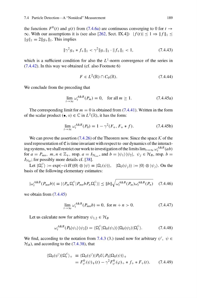
the functions F
0
(t) and g(t) from (7.4.6a) are continuous converging to 0 for t →
∞. With our assumptions it is (see also [262, Sect. IX.4]) | f (t)| ≤ 1 ⇒ ⇒ f 1 ≤
g 1 = 2g + 1 . This implies
γ
2
g + ∗ f + 1 < γ
2
g + 1 · · f + 1 < 1,
(7.4.43)
which is a sufficient condition for also the L
1 -norm convergence of the series in
(7.4.42). In this way we obtained (cf. also Footnote 6)
F ∈ L
2
(R) ∩ C 0 (R).
(7.4.44)
We conclude from the preceding that
lim
t→∞
ω
A&B
t
(P m ) = 0, for all m ≥ 1.
(7.4.45a)
The corresponding limit for m = 0 is obtained from (7.4.41). Written in the form
of the scalar product (•, ◦) ∈ C in L
2
(R), it has the form:
lim
t→∞
ω
A&B
t
(P 0 ) = 1 − γ
2
(F + , F + ∗ f ).
(7.4.45b)
We can prove the assertion (7.4.26) of the Theorem now. Since the space K of the
used representation of C is time invariant with respect to our dynamics of the interacting systems, we shall restrict our work to investigation of the limits lim t→∞ ω
A&B
t
(ab)
for a = P mn , m, n ∈ Z + , resp. a = I H vac , and b = |ψ 1 ψ 2 |, ψ j ∈ H B , resp. b =
I H B ; for possibly more details cf. [38].
Let |
ψ
t := exp(−it H)|0 ⊗ |ψ ≡ | t (ψ), | 0 (ψ j ) := |0 ⊗ |ψ j . On the
basis of the following elementary estimates:
|ω
A&B
t
(P mn b)| ≡ ||P m
ψ
t |P mn bP n
ψ
t | ≤ ≤b
ω
A&B
t
(P m )ω
A&B
t
(P n ) (7.4.46)
we obtain from (7.4.45)
lim
t→∞
ω
A&B
t
(P mn b) = 0, for m + n > 0.
(7.4.47)
Let us calculate now for arbitrary ψ 1,2 ∈ H B
ω
A&B
t
(P 0 |ψ 1 ψ 2 |) = =
ψ
t | 0 (ψ 1 ) 0 (ψ 2 )|
ψ
t .
(7.4.48)
We find, according to the notation from 7.4.3 (3.) (used now for arbitrary ψ
, ψ ∈
H B ), and according to the (7.4.38), that
0 (ψ
)|
ψ
t + ≡ ≡ 0 (ψ
)|P 0 U t P 0 | 0 (ψ) +
= F
0
ψ (ψ) + (t) − γ
2 F
0
ψ (ϕ) + ∗ f + ∗ F + (t).
(7.4.49)
189
the functions F
0
(t) and g(t) from (7.4.6a) are continuous converging to 0 for t →
∞. With our assumptions it is (see also [262, Sect. IX.4]) | f (t)| ≤ 1 ⇒ ⇒ f 1 ≤
g 1 = 2g + 1 . This implies
γ
2
g + ∗ f + 1 < γ
2
g + 1 · · f + 1 < 1,
(7.4.43)
which is a sufficient condition for also the L
1 -norm convergence of the series in
(7.4.42). In this way we obtained (cf. also Footnote 6)
F ∈ L
2
(R) ∩ C 0 (R).
(7.4.44)
We conclude from the preceding that
lim
t→∞
ω
A&B
t
(P m ) = 0, for all m ≥ 1.
(7.4.45a)
The corresponding limit for m = 0 is obtained from (7.4.41). Written in the form
of the scalar product (•, ◦) ∈ C in L
2
(R), it has the form:
lim
t→∞
ω
A&B
t
(P 0 ) = 1 − γ
2
(F + , F + ∗ f ).
(7.4.45b)
We can prove the assertion (7.4.26) of the Theorem now. Since the space K of the
used representation of C is time invariant with respect to our dynamics of the interacting systems, we shall restrict our work to investigation of the limits lim t→∞ ω
A&B
t
(ab)
for a = P mn , m, n ∈ Z + , resp. a = I H vac , and b = |ψ 1 ψ 2 |, ψ j ∈ H B , resp. b =
I H B ; for possibly more details cf. [38].
Let |
ψ
t := exp(−it H)|0 ⊗ |ψ ≡ | t (ψ), | 0 (ψ j ) := |0 ⊗ |ψ j . On the
basis of the following elementary estimates:
|ω
A&B
t
(P mn b)| ≡ ||P m
ψ
t |P mn bP n
ψ
t | ≤ ≤b
ω
A&B
t
(P m )ω
A&B
t
(P n ) (7.4.46)
we obtain from (7.4.45)
lim
t→∞
ω
A&B
t
(P mn b) = 0, for m + n > 0.
(7.4.47)
Let us calculate now for arbitrary ψ 1,2 ∈ H B
ω
A&B
t
(P 0 |ψ 1 ψ 2 |) = =
ψ
t | 0 (ψ 1 ) 0 (ψ 2 )|
ψ
t .
(7.4.48)
We find, according to the notation from 7.4.3 (3.) (used now for arbitrary ψ
, ψ ∈
H B ), and according to the (7.4.38), that
0 (ψ
)|
ψ
t + ≡ ≡ 0 (ψ
)|P 0 U t P 0 | 0 (ψ) +
= F
0
ψ (ψ) + (t) − γ
2 F
0
ψ (ϕ) + ∗ f + ∗ F + (t).
(7.4.49)